Autonomous Vehicle Projects: PID Control for Vehicle Steering

Control systems in autonomous vehicles are used to direct various hardware, including steering wheels, throttle, and brakes among others. These systems take outputs from a path planning system (such as a target velocity in a cruise control) and execute them on the vehicle’s hardware. While humans drivers can easily steer, use the accelerator and brake pedals to safely drive their cars, control systems in autonomous vehicles can be quite challenging to implement for safe, efficient, and pleasant driving.

A Proportional-Integral-Derivative controller, or PID controller for short, is a mechanism which is very common for various applications requiring continuous control changes in autonomous vehicles. By calculating the error between the current and desired value of a control (for example, the angle of the steering wheel), a PID controller applies a correction to smoothly approach the desired value of the control itself.

This repository contains a software system which steers a vehicle around a simulated track using a PID controller. The following techniques are used:

  • Apply a PID controller for steering
  • Use a training module to implement coordinate descent for PID parameter optimization

Exploring my implementation

All of the code and resources used in this project are available in my Github repository. Enjoy!

Technologies Used

  • C++
  • uWebSockets

PID Controllers

Many control environments account for both a) a desired setting for a control (such as a target speed in a cruise control or a target vehicle heading from an autonomous vehicle path planner), as well as b) external forces which may change the value of the control (such as a hill or bumpy road which slows down a vehicle’s forward movement). To allow the vehicle to track a target control value, PID controllers repeatedly compute the error between a measurement of a process variable (which contains current value of the control) and the desired setpoint (what the value of the control should be). Then, the controller applies a correction based on the proportional, integral, and derivative parameters of the controller. This allows the vehicle to approach the desired value of the control (such as the target speed) in an efficient way, both quickly and without overshoot.

PID smooth

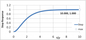
In the image above, the target value of 1 is approached rapidly and smoothly.

The proportional correction adjusts the value of the control in proportion to the difference between the target value and the actual value. For example, if the target speed is 50mph, the proportional correction will be double at a current speed of 40mph (difference of 10mph) than what the correction will be at a current speed of 45mph (difference of 5mph).

The integral correction adjusts the value of the control to account for any constant misalignment between the control output and the hardware. For example, a non-centered steering wheel alignment in vehicles can yield a centered steering wheel which does not guide the vehicle in straight line; the integral correction accounts for this misalignment.

The differential correction adjusts the value of the control to prevent overshooting the target value. Without this, the proportional control would only reduce the control value to zero once the target has been reached; but in true situations, the control value should be reduced to zero to “coast” to the target value in the last moments.

PID overshoot

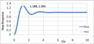
Note how in the image above, the target value of 1 is overshot several times before the actual value settles at the target. A properly adjusted differential correction prevents this.

Implementation

PID controller

The PID controller in this repository is responsible for controlling the steering angle of the vehicle to keep it in the center of the driving lane. To do this, the error used in the PID controller for correction is the cross-track error, which is the distance between the vehicle and the center of the lane. If the vehicle is exactly in the lane center, then the error is zero.

The PID controller for steering is implemented in a standard fashion, with error adjustments based on the sum of:

  • current error proportional to a constant (proportional)
  • total error summed over each step proportional to a constant (integral)
  • error delta since previous step proportional to a constant (differential)

Training module

A training module is implemented to optimize the PID parameters based on the coordinate descent algorithm. The algorithm optimizes each parameter in the error function independently, moving it up or down to find a small improvement in error. This method will find the local minima of the error function overall, meaning that the parameters found are not guaranteed to be the best parameters to minimize error, but will be based on starting parameters given.

The coordinate descent algorithm is embedded in a framework to ensure that the total error measurement for parameter setting ends up taking the entire track into account, not just a small portion of it. However, small portions of track are useful for initial parameter and parameter delta setting in the early moments of the algorithm run, to prevent the vehicle from leaving the drivable portion of the track surface. The training module ensures that if the vehicle appears to be leaving the track surface, the last best parameters are re-installed in the PID controller temporarily, until the vehicle returns to a safe driving state. In that case, those particular parameters that caused the vehicle to lose control are then invalidated as candidates for possible best selection, even if their overall error rate was lower than the previous best error rate.

Results

Using the training module, and with the initial parameters of p = 0.1, i = 0.01, d = 1.0, the training module arrived at a local minima of error with final parameter values p = 0.127777, i = 0.00937592, d = 1.03501 (in the Linux simulator) and p = 0.3011, i = 0.00110, d = 4.8013 (in the Mac simulator). The two simulators provide different data (different vehicle timestep sizes and angles) to the control program; hence, different values are necessary.

The proportional steering control ensures that steering corrections are proportional to the error at each timestep. It is easy to verify this on its own; when the vehicle is travelling away from the center of the lane, the steering commands direct the vehicle back toward the center. However, with this value set and the integral and differential values at zero, the vehicle sways wildely back and forth through the track.

The integral steering control corrects for steering bias of the vehicle. The vehicle naturally “pulls” to the side when the steering command is 0.0; this ensures that the vehicle drives relatively straight when it is in the center of the lane.

The differential steering control attempts to limit the wild sway of the vehicle as it corrects errors by counter-steering. As steering is changed to correct for error, adjustments are reduced by the amount of change between each time step in the simulation. This attempts to prevent the vehicle from overshooting the center of the lane during a correction.

Overall, these settings for the PID controller ensure that the vehicle drives continuously around the track without hitting any road hazards or leaving the drivable portion of the road surface. One caveat is that in the first few seconds of driving, while the vehicle is under 30 mph, the vehicle does sway from side to side.

Read More

Autonomous Vehicle Technology: Localization using Particle Filters

In order to drive safely, autonomous vehicles on public roads need to know where they are in the world. Tasks easy for humans, such as staying in driving lanes at all times, would be impossible for an autonomous vehicle to perform without highly accurate vehicle location information. Determining the vehicle’s location in the world is called localization. One popular and well-known localization system is the global positioning system (GPS), which can provide rough localization; it often has accuracy of one to three meters, but the accuracy can decrease to upwards of fifty meters with poor line off sight to the sky or other interference. Unfortunately, this is not accurate enough for an autonomous vehicle; a localization accuracy of under ten centimeters is considered the upper limit for safe driving.

Like the techniques involved in object tracking using extended and unscented Kalman filters, localization techniques are often probabilistic. The unscented Kalman filter is flexible enough for many object tracking applications; however, when even higher accuracy is required for vehicle localization, another technique can be used: a particle filter.


Exploring my implementation

All of the code and resources used in this project are available in my Github repository. Enjoy!

Technologies Used

  • C++
  • uWebSocketIO

Particle Filters

Particle filters are similar to unscented Kalman filters in that they update the state of an object (for example, the location and orientation) by transforming a set of points through a function to predict a future state, given noisy and partial observations of the world. However, unlike unscented Kalman filters, particle filters may choose points to transform at random, rather than from a Gaussian distribution. This eliminates the need to assume a static state motion or measurement model. The number of points required for a particle filter to obtain the same level of accuracy as an unscented Kalman filter is generally higher, which makes a particle filter more computationally complex and memory intensive. Additionally, there is a choice to be made regarding the number of particles included in the filter (the time complexity of computing the algorithm is linear in the number of particles). However, particle filters do converge to the true state of the object being predicted as number of particles increases, unlike unscented Kalman filters, which have no such convergence properties.

Particle filter steps

In a particle filter, the points, or “particles”, are chosen to represent concrete guesses as to the actual state being predicted. At each time step, particles are randomly sampled from the state space. The probability of a particle being chosen is proportional to the probablility of it being the correct state, given the sensor measurements seen so far. The update step in a particle filter can be seen as selecting the most likely hypotheses among the set of guessed states; as more sensor measurements become available, those more likely to be true are kept, while those less likely are removed.

Particle filters for localization

When used for localization, particle filters become a particularly effective technique. Because they can approximate non-parametric functions, they perform better in many non-linear model environments, including situations with multiple possible localization positions. For example, when using a Kalman filter (extended or unscented), a vehicle driving down a road with many similar lampposts may decide that it is next to a lamppost, but may have trouble determining which lamppost it is next to.

In using a particle filter for localization, data from onboard sensors (such as radar and lidar) can be used to measure distances to static objects (trees, poles, walls), which may involve sensor fusion. With a pre-loaded map which has trusted coordinates of these fixed objects, a particle filter matches observations of objects in the world against those in the map, and then determines where the vehicle is in the map space. To start, particles may initially be chosen at random from all locations, with no assumptions about where the vehicle is. However, in practice, some sort of one-time hint about the general location from GPS may be provided. At each time step, the algorithm uses its previous belief about vehicle location, the current vehicle control values, and sensor measurements, and outputs a new belief about the vehicle location.

The algorithm runs by updating the current set of particles (possible locations) according to the vehicle control command, simulating motion of all of the particles. For instance, if the vehicle is travelling forward, all particles move forward. If the vehicle turns to the right, all of the particles turn to the right. Because the result of a control does not always complete as expected, some amount of noise is added to the particle movement to simulate this uncertainty. Each particle is then considered to be the possible location of the vehicle, and the probability that the location is the true location of the vehicle given the current sensor measurements is computed. Those probabilities are used as weights to randomly select new particles from the previous particle list. Because of this, particles which are consistent with sensor measurements are more likely to be chosen (and may even be chosen more than once!), and particles which are inconsisent with the measurements are less likely to be chosen. However, to prevent convergence on an incorrect location (if the vehicle is stationary, for instance), extra uniformly sampled particles can be added.

With every iteration of the particle filter algorithm, the selected particles converge to the true location of the vehicle, which makes intuitive sense: as the vehicle senses more of its environment, it should be expected to become increasingly sure of its position.

Localization maze

Implementation

The localization algorithm exists as a loop, where new sensor measurements and control commands are read. On the first sensor measurement, the particle filter is initialized with that measurement; on subsequent measurements, the particle filter is run to predict the new location of the vehicle. Next, the particles have their weights updated using observations from sensors and known map landmarks, then particles are resampled. Finally, the particle with the highest weight is chosen as the new location of the vehicle.

Inside the particle filter, the initialization step creates 100 particles, locates them all at the first measurement, and then adjusts each particle randomly according to the sensor measurement uncertainty distribution. During prediction, each particle’s next location is predicted by moving it according to the velocity and turn rate from most recent vehicle control command.

To update the weights for each particle based on the sensor observations of landmarks, the landmarks nearest the particle are chosen. Next, each observation is paired with its closest true landmark. Finally, the particle’s weight is set to the product of the distance between each true landmark and its closest observation.

Particle resampling occurs according to the particles weights, which is a standard sampling with replacement approach.

Performance

To test the localization using the particle filter, the simulator provides sensor measurements of fixed objects in the world. These are plotted in the simulator as black crosses with circles around them. Green lines drawn between the vehicle and the circles indicate fixed objects which are being tracked.

The jitter between the vehicle (true location) and the grey circle (predicted location) is kept to a relative minimum over time, even during accelerations, decelerations, and turns. This indicates that the filter does a relatively good job at localization.

Read More