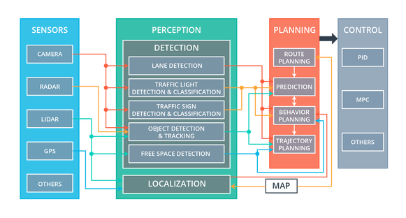
The self-driving systems in autonomous vehicles have four major components: sensors, perception software, planning software, and control software. Within each of the software components, multiple modules execute concurrently to process vast amounts of data collected from the sensor systems. This processing eventually results in control outputs which steer, accelerate, and brake the vehicle at the right moments to get the vehicle safely and efficiently to its destination while providing a pleasant ride for its passengers.
Each of these systems in an autonomous vehicle operate with input from upstream components: for example, the lane detection module might input data from a camera; the localization system might input data from a lidar and gps module; and the vehicle behavior prediction module might input data from the lane detection, traffic light detection, traffic sign classification, and object detection and tracking systems. An example data flow graph between all of the software modules in an autonomous vehicle might look like this:
Wiring up all of the various inputs and outputs from each module, given the different types of data and refresh rates provided by each module, is non-trivial and time-consuming. Using a software framework specifically designed for this, the Robot Operating System (or ROS for short), can make this challenge significantly easier, by abstracting away hardware details, managing data flow between software modules, and hosting common re-usable code.
Together with several other team members, I implemented a completely autonomous vehicle software system (including perception, planning, and control) using ROS, which was then used to run on a real-life Lincoln MKZ hybrid vehicle to autonomously drive around a test lot.
Exploring my implementation
All of the code and resources used in this project are available in our team’s Github repository. Enjoy!
Technologies Used
- C++
- Python
- ROS
- Flask
- Keras
- Tensorflow
- NumPy
- SciPy
- Python Imaging Library
- OpenCV
System Integration with ROS
Autonomous Vehicle Systems
Within an autonomous vehicle, each vehicle component has a specific task:
Sensors are the hardware components that gather raw data about the environment. They include LIDAR, RADAR, cameras, and even GPS sensors.
Perception systems (including detection and localization components) process raw sensor data into meaningful structured information about the environment around a vehicle. The detection components are responsible for lane line detection, traffic sign and light detection and classification, object detection and tracking and free space detection. Localization components use sensor and map data to determine the vehicle’s precise location.
Planning systems use the output from the perception systems to create driving behaviors and to plan short and long-term paths for the vehicle to follow. Planning components include high-level route planning from start to destination on a map, prediction of what other objects on the road might do, behavior planning to decide what specific actions the vehicle should take next, and trajectory generation which plots the precise path the vehicle should follow.
Control systems ensure that the vehicle follows the path given by the planning system and send commands to the vehicle’s hardware for safe driving. These include sending acceleration, braking, and steering commands.
Information generally flows from top to bottom, starting with sensor systems, then moving through perception, planning, and finally to control systems.
System integration
ROS is an open-source robotics framework which solves many of the challenges of communication and modularity that come with integrating all of these vehicle systems. It is widely used in industry and academia and provides libraries and tools for common tasks involving transferring data between modules, dealing with sensor and control actuator interaction, logging, error handling, process scheduling, and interfacing with common third-party libraries. Visualization, simulation, and data analysis tools are also provided, which are incredibly useful for building and debugging a completely autonomous vehicle. Altogether, ROS lets autonomous vehicle engineers focus on the algorithms they wish to implement for each module rather than spending time on the “glue” that holds the entire system together.
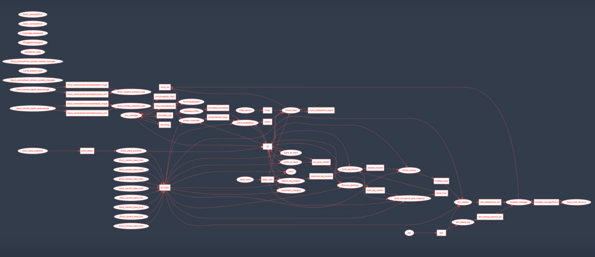
An autonomous vehicle system in ROS is built by writing perception, planning, and control algorithms into modules called nodes, which are containers for algorithms. Nodes are designed to be lightweight and focused one specific task; each sensor, perception component, planning component and actuator may have its own node. A special node, called the ROS master, manages all nodes and facilitates communication between them. It allows nodes to identify each other, communicate, and to listen for and request parameters, which are ways to tune each node’s behavior quickly and easily. An autonomous vehicle may have hundreds of nodes, depending on the complexity of the vehicle being controlled.
Here is a graph of the nodes in a moderately complex robot:
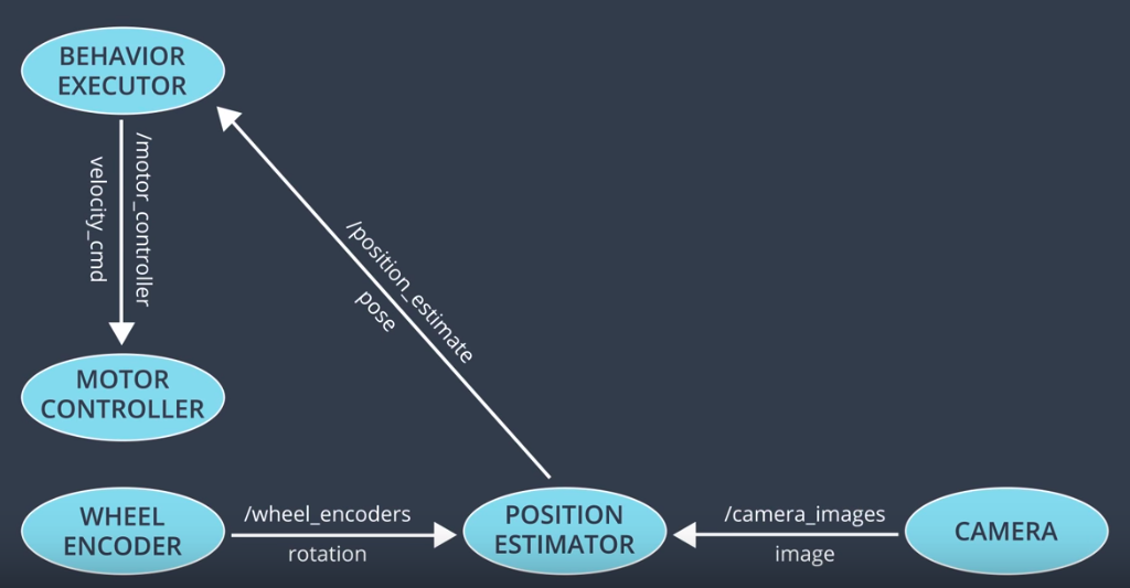
Nodes share data with each other by using message passing on topics, whose messages are being read by one or more nodes. For example, a lidar node may write a new sensor measurement to a lidar topic, and the message will be read by all nodes which subscribe to that topic, for example, a free-space detection node and a localization node. ROS comes with many different message types, which are useful for sending data typically associated with autonomous vehicles: sensor measurements, steering wheel angles, images, point clouds, and custom message types that developers can create.
Here is a small graph of nodes and the types of messages that they send:
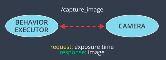
Sometimes, having a system which can listen for requests and respond to them is useful; ROS supports services which do precisely this. Services operate in much the way that a typical web service waits for a request, processes the input, computes a response, then sends it back to the requestor. For example, a camera node would publish many images per second on a camera topic (for any subscribers who may be listening), but if a behavior planner only wants to process an image from a camera every few seconds, then a camera service would be useful to return the current camera image that is available.
Training Dataset
A training dataset was prepared by combining simulator data with data provided by other vehicles which ran on the test track.
Implementation
Together with several other team members, I implemented a completely autonomous vehicle software system (including perception, path planning, and control) using the ROS framework, which was then used to run on a real-life Lincoln MKZ hybrid vehicle to autonomously drive around a test lot.
The real vehicle has a Dataspeed drive-by-wire (DBW) interface for throttle, brake, and steering control, a forward-facing camera for traffic light detection, and LIDAR for localization. Autonomous vehicle software is run on a Linux PC with ROS and a TitanX GPU for TensorFlow processing.
Development proceeded using a local simulator, after which successful testing proceeded to a real-life vehicle in a test lot.
System Architecture
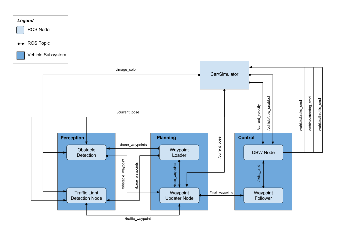
The autonomous vehicle system starts by loading mapped route base waypoints (locations to follow on the test track) in the planning system’s Waypoint Loader and setting an overall maximum speed guard for each waypoint. This initial setup is used to protect for safe operation in the test lot.
The system then starts receiving the vehicle’s sensor data: current pose from LIDAR localization, current speed, DBW enable switch and camera images.
The perception system’s Traffic Light Detection Node processes camera images to detect traffic lights, and to decide if and where the vehicle needs to stop at an upcoming waypoint location.
The planning system’s Waypoint Updater Node plans the driving path target speed profile by setting upcoming waypoints with associated target speeds. This includes smoothly accelerating up to the target maximum speed and slowing down to stop at detected red lights. This is accomplished by using a smooth speed profile planner using a Jerk Minimizing Trajectory (JMT) following dynamic red light stopping locations.
The control system’s Waypoint Follower sets target linear speed (from the planned waypoint target speeds) and target angular velocity to steer toward the waypoint path.
The control system’s Drive-By-Wire Node computes throttle, brake, and steering commands using PID feedback control for throttle and brake, and a kinematic bicycle model yaw control for steering, both of which are then low-pass filtered to eliminate rapid back-and-forth control changes. These commands are sent to the Dataspeed drive-by-wire system to actuate the vehicle’s pedals and steering wheel.
Traffic light detection
A teammate worked on this module; their description of their work is adapted here.
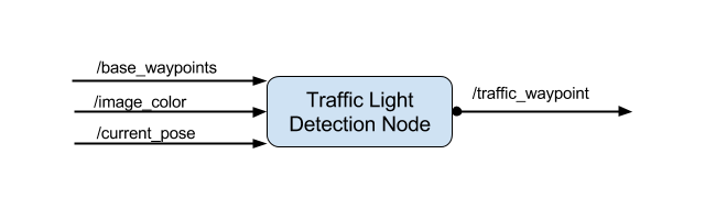
The traffic light detection node subscribes to the following topics:
- image_color provides an image stream from the vehicle’s camera. These images are used to determine the color of upcoming traffic lights
- current_pose provides the vehicle’s current position
- base_waypoints provides a complete list of waypoints of the vehicle’s course
- vehicle/traffic_lights provides the (x, y, z) coordinates of all traffic lights. This helps to acquire an accurate ground truth data source for the traffic light classifier by sending the current color state of all traffic lights in the simulator for testing purposes, before running on the real vehicle
The node publishes the index of the waypoint for the nearest upcoming red traffic light’s stop line to the traffic_waypoint topic.
The camera image data is used to classify the color of the upcoming traffic light using a classifier.
Traffic Light Classifier
Architecture
A classifier was built using transfer learning on a ResNet50 convolutional neural net architecture. This pre-trained Keras model was previously trained on the ImageNet dataset. The first 150 layers of the model were frozen, and the top layers were removed. One average pooling layer, one fully connected layer with ReLU activation, two dropout layers, and one softmax loss layer with four classes (Green, None, Red, Yellow) were added. An Adam optimizer was used during the training with a low learning rate (0.00001).
Training Dataset
A training dataset was prepared by combining simulator data with data provided by other vehicles which ran on the test track.
Preprocessing
To pre-process input data, training images were resized to (224,224) which is the input to ResNet50 architecture. Next, the images were randomly adjusted to images seen the camera in true driving conditions, by:
- rotation by a random angle (+/- 5 degrees)
- random horizontal flipping
- random zooming (+/- 0.3)
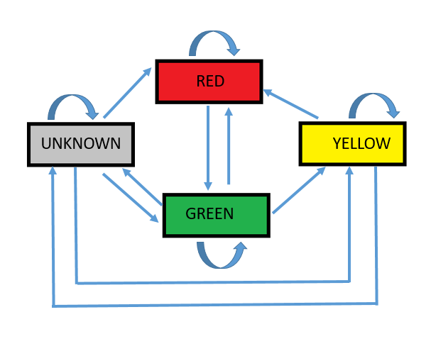
Traffic Light Detection State Machine
The determination of the color of the traffic light is made based on a state machine which uses the previous light state information to determine the allowed light states and compare it with the classified light state. Each predicted state has to be predicted several of times before it becomes trusted as the correct state of the traffic light. If the classified light state does not match with any of the allowed light states, then the light state does not change.
Closest Waypoint
The base waypoints provide the complete list of waypoints for the course. Using the vehicle’s current location and the coordinates for the traffic lights, the nearest visible traffic light ahead of the vehicle is identified. The closest waypoint index is published to the waypoint updater node if the vehicle is approaching nearest light.
Waypoint Updater
A teammate worked on this module; their description of their work is described here.
The waypoint updater node has two main tasks:
- Waypoint preparation – Load the waypoints from the /base_waypoints topic and prepare them for use during planning
- Planning
- Use pose messages from /current_pose topic to identify the location of the closest waypoint in front of the vehicle
- Use messages from /traffic_waypoint topic to decide whether the vehicle should speed up, maintain current speed, or come to a stop. Also, it should calculate an appropriate trajectory to accomplish this. A set of waypoints and velocities is then published to the /final_waypoints topic for the waypoint follower to consume
Trajectory Velocity Calculations
Jerk minimizing trajectory planning is used to produce speedup and slowdown profiles that can be merged at any point based on changing traffic signal status without exceeding 10m/s^2 of acceleration or 10 m/s^3 of jerk, which would cause passenger discomfort.
Loading the Waypoints
The waypoints are loaded into a custom structure which stores the waypoint data, the distance of the waypoint (through preceding waypoints) from the start of the track, the maximum velocity allowed for that waypoint, and the velocity, acceleration, jerk, and elapsed time variables used in the jerk minimizing trajectory planning calculations.
The vehicle coordinates of each of the waypoints are also loaded into a kd-tree to enable finding the closest waypoint to the vehicle. This search is used as a backup method to find the closest waypoint. Tests have shown the kd-tree to be very fast and usable for up to at least 11,000 waypoints; however, it is generally only used by the waypoint_updater at startup.
Once the waypoints have been loaded and at least one pose message has been received, the updater loop begins. The loop is set to run at approximately 30 Hz.
Trajectory Planning
The first stage uses the most recent pose data to locate the closest waypoint ahead of the vehicle on the waypoint list. Since the vehicle is expected to follow the waypoints, a local search of waypoints ahead and behind the waypoint identified in the last cycle is conducted to try to find the vehicle location as quickly as possible.
A check is then made to see if a traffic_light message has been received from the traffic light detection system since the last cycle. Messages are stored and only updated at the start of each cycle to prevent race conditions when the traffic signal information changes during an ongoing cycle.
The vehicle can be in one of five states:
- Stopped – the vehicle is not moving and is waiting at a red or yellow light
- Creeping – the vehicle is moving at a steady minimum velocity up to a stop line
- Speedup – the vehicle is accelerating toward the default cruising velocity
- Maintainspeed – the vehicle is maintaining constant default cruising speed
- Slowdown – the vehicle is decelerating to stop just behind the stop line
If the vehicle is moving (in speedup,maintainspeed, or slowdown states), the minimum stopping distances are calculated to prevent exceeding maximum desired jerk and maximum allowed jerk using the current velocity and acceleration of the vehicle as starting conditions. This remains an area of investigation, as a simple, fast and accurate method to determine the minimum distance required to prevent exceeding a specific jerk level has not been achieved. The current method is functional but is thought to overestimate the necessary distance. This is a critical issue, as it is key in the decision as to whether the vehicle can stop for a signal.
During tests on in simulator, it was found that the minimum stopping distance calculated at higher speeds (~ 60 m for 60 km/hr) to meet maximum jerk limits occasionally resulted in not being able to stop for a red traffic light which was detected within 60m of the line. At 40 km/hr the minimum stopping distance was below 30m which could still result in the vehicle going through a yellow light but was much less likely to result in moving through a red light. The slower speed also gave more time for the traffic light classifier to operate.
If the distance to a signaling light is between the two calculated stopping distances, the time required to complete the slowdown is optimized to produce the lowest jerk along the trajectory, and the slowdown trajectory is calculated and published. If the distance to the traffic light is greater than the larger stopping distance, then the vehicle will continue on its current plan. If the distance to the traffic light is less than the minimum calculated stopping distance, then the planner will proceed past the signal – this should correspond to driving through a yellow light.
A decelerating message is published when the planner has put the vehicle in slowdown or stopped to assist the DBW Node with braking control.
In the event that the vehicle is in slowdown or stopped, and the distance to the next signaling traffic light increases beyond the calculated stopping distance, a new trajectory is calculated to accelerate the vehicle to the default velocity. Maximum desired jerk is used as the criteria to calculate the distance and time over which this trajectory should be completed. This algorithm is not optimal, but overestimating the minimum distance required to accelerate without exceeding a specific jerk limit is not as critical as being able to stop in time for a stop signal.
A special creeping state was used for the condition where the vehicle is stopped a short distance from a stop signal. If the vehicle is within the creeping setback from the light, the planner will just use the minimum moving velocity on waypoints until the vehicle gets to the traffic light buffer setback, where velocity is returned to zero. This prevents short acceleration/braking cycles at the light, simulating a driver just releasing the brake to ease forward.
The upcoming waypoints are published to the /final_waypoints topic. It was found that using 40 waypoints in the simulator was sufficient for use by the waypoint follower.
The calculation time required in each cycle was low enough in the conditions tested that no algorithm was necessary to account for latency when publishing the waypoints.
Waypoint Follower
A teammate worked on this module; their description of their work is described here.
In order to drive along the planned path consisting of waypoints with associated target speeds and yaw angles, an implementation of the Pure Pursuit algorithm is used.
This algorithm receives the upcoming waypoints from the Waypoint Updater and publishes a target linear velocity and angular velocity for the DBW Node to control throttle, brake, and steering actuators.
Pure Pursuit Algorithm Overview
The Pure Pursuit algorithm finds the radius of a circular path that is tangent to the current orientation of the vehicle and crosses through a point on the target driving path some distance ahead (called “the look-ahead point”), then calculates the corresponding target angular velocity to follow it. As the vehicle drives forward and steers along this arc, the look-ahead point continues to be pushed further ahead so the vehicle gradually approaches and straightens along the path.
The amount of look-ahead distance alters the sharpness of the steering angles, where a short look ahead causes larger steering angles but can follow sharp turns, and a large look ahead causes smaller steering angles but may cut the corners of the driving path. The look-ahead distance is variable in proportion to the vehicle speed.
The target linear velocity from this algorithm passes through the target velocity associated with the closest waypoint.
Autoware Open-source Pure Pursuit Library
The Autoware open-source ROS module called “Waypoint Follower” has been included to perform the pure pursuit algorithm. However, the base C++ algorithm had some areas that needed further improvement:
- Tuned the judgment thresholds for distance and relative angle thresholds to keep more continuous steering adjustments to prevent ping-ponging around the target path
- Perform closest waypoint search to pick up the correct waypoint speed targets when the vehicle has driven past the initial waypoints in the list (in case of lag or Waypoint Follower updating at a faster rate than Waypoint Updater)
- Perform look-ahead waypoint search starting from the closest waypoint instead of the initial waypoint in the list to prevent searching far behind the vehicle
- Tune the minimum look-ahead distance to be able to steer around tighter turns (such as the test lot)
- Fix the possibility for negative target velocity command at high lateral velocities
Drive-By-Wire Node
The autonomous vehicle for which this system was written uses a Dataspeed drive-by-wire interface. The interface accepts a variety of control commands, including (but not limited to):
- throttle – for pedal position
- brake – for braking torque (or pedal position)
- steering – for steering wheel angle
The job of the DBW control node in this software is to publish appropriate values to these three control command interfaces, based on input from upstream message sources:
- twist_cmd – target linear and angular velocity published by the waypoint follower
- current_velocity – current linear velocity published by the vehicle’s sensor system
- dbw_enabled – flag indicating if the drive-by-wire system is currently engaged
- is_decelerating – flag indicating if the waypoint updater is attempting to decelerate the vehicle
ROS Node
The main DBW ROS node performs the following setup upon being created:
- accepts a number of vehicle parameters from the vehicle configuration
- implements the dbw_node ROS topic publishers and subscribers
- the four ROS topic subscribers (twist_cmd, current_velocity, dbw_enabled, is_decelerating) assign various instance variables, used by the Control class, once extracted from the topic messages
- creates a Controller instance to manage the specific vehicle control
- enters a loop which provides the most recent data from topic subscribers to the Controller instance
The loop executes at a target rate of 50Hz (any lower than this and the vehicle will automatically disable the DBW control interface for safety). The loop checks if the DBW node is enabled, and all necessary data is available for the Controller, then hands the appropriate values (current and target linear velocity, target angular velocity, and whether the vehicle is attempting to decelerate) to the Controller. Once the Controller returns throttle, brake, and steering commands, these are published on the corresponding ROS interfaces.
Controller
A Controller class manages the computation of throttle, brake, and steering control values. The controller has two main components: speed control and steering control.
The Controller, upon initialization, sets up a Yaw Controller instance for computing steering measurements, as well as three Low Pass Filter instances for throttle, brake, and steering.
Speed control
At each control request, the following steps are performed:
- Compute the timestep from the last control request to the current one
- Compute the linear velocity error (the difference between target and current linear velocity)
- Reset PI control integrators if the vehicle is stopped (has a zero target and current linear velocity); more on the integrators later
Next, the raw throttle and brake values are computed. The basic design:
- adds variable throttle if the vehicle is accelerating or vehicle is slowing down but not significantly enough to release the throttle entirely
- adds variable braking if the vehicle is traveling too fast relative to the target speed (and simply releasing throttle will not slow down fast enough)
- adds constant braking if the vehicle is slowing down to a stop
Once the raw throttle and braking values are computed, the raw braking value is sent through a low pass filter to prevent rapid braking spikes. If the resulting value is too small (below 10Nm), the braking value is reduced to zero; else, the throttle is reduced to zero. This is to prevent the brake and throttle from actuating at the same time. Finally, the throttle value is sent through a separate low pass filter to prevent rapid throttle spikes.
Steering control
The target linear velocity, target angular velocity, and current linear velocity are sent into the Yaw controller. This controller computes a nominal steering angle based on a simple kinematic bicycle model. Finally, this steering value is sent through its own low pass filter to smooth out final steering commands.
Visualization Tools
A teammate worked on this module; their description of their work is described here.
Some visualization tools were built for monitoring data while running the simulation using the ROS tools RQT and RViz.
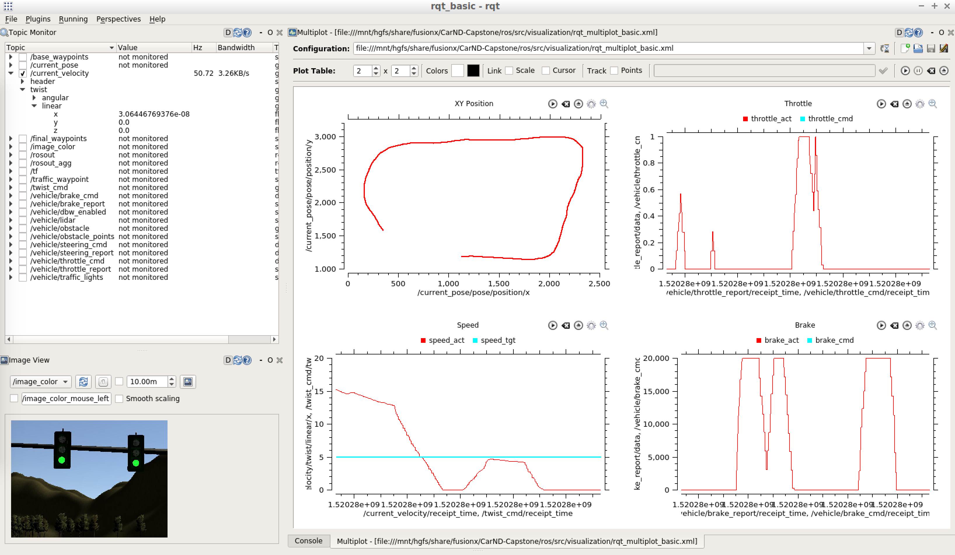
RQT
Here is a sample of the RQT view including dynamic parameters, xy position on the track, throttle, speed, and braking values.
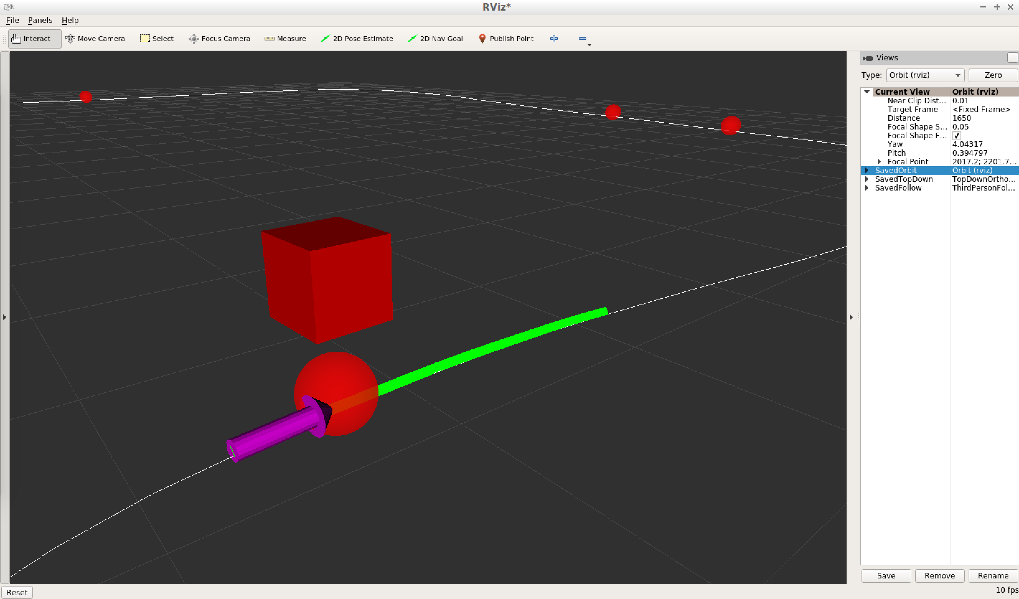
RViz (3D scene view)
To visualize the vehicle’s position relative to the waypoints and traffic lights in an RViz 3D scene, a visualization node is used to publish a /visualization_marker_array topic to populate the objects and a /visualization_basewp_path topic to populate a path line.
The visualization node publishes when the parameter vis_enabled == True. When using the actual vehicle, the visualization node is not launched to reduce bandwidth.
Here is a sample view of the RViz 3D scene view:
Testing
Testing the fully integrated system proceeded in multiple ways. First, the traffic light classifier was tested and debugged with real-world camera images. Once complete, the fully integrated system was run locally against a vehicle simulation on a highway track and a test lot. The data visualization and analysis tools helped to find issues and correct them as they appeared.
This video shows a successful run of the vehicle in the simulator:
Results
For the final test, the fully integrated system was loaded onto a real vehicle to run in a simulated test lot. After several testing and debugging iterations, the final test was a complete success. The vehicle was piloted up to a traffic light, where it stopped for a red light, then proceeded on a green. It drove very smoothly with appropriate acceleration around the test track and followed the route around the test lot without difficulty.