Control systems in autonomous vehicles are used to direct various hardware actuators, including steering wheels, throttle, and brakes among others. These systems take command outputs from a path planning system (such as a target velocity in a cruise control) and execute them on the vehicle’s hardware. While humans drivers can easily steer, use the accelerator and brake pedals to safely drive their cars, control systems in autonomous vehicles can be quite challenging to implement for safe, efficient, and pleasant driving.

One approach to creating a high-quality controller for an autonomous vehicle is to model the vehicle’s dynamics and constraints; this allows for easier analysis and tuning of the controller itself. Model Predictive Control (MPC) is an advanced technique used to control one or more hardware actuators, making optimal control choices for both the present circumstances and the future; for example, when given a trajectory from a path planner. By modeling the dynamics of the vehicle through time, and including explicit constraints on the vehicle dynamics, a MPC can control complex actuators in a much more flexible manner than a PID controller.

This repository contains a software system which implements a MPC for steering and throttle of a vehicle around a simulated track, given a path from a planner.

Exploring my implementation

All of the code and resources used in this project are available in my Github repository. Enjoy!

Technologies Used

• C++
• uWebSockets
• Eigen
• C++ Algorithmic Differentiation (CppAD)
• Interior Point Optimizer (IPOPT)

Model Predictive Control

Model predictive control shows its strengths when used with moderate to complex systems (like the movement of an autonomous vehicle) that can be linearly modeled or considered approximately linear over a small operating range or timescale.

Vehicle modeling

A basic model for a vehicle is a kinematic model, which captures position, heading, and speed, and ignores many elements like gravity, mass, and tire forces. It is simple and often works well for vehicles moving at low and moderate speeds. Dynamic models can capture a much more rich state of a vehicle such as tire forces, air resistance, gravity, drag, and longitudinal and lateral forces. While dynamic models can more accurately represent how a vehicle moves, basic models have two main advantages: they require less computational resources (making them easier to execute in real-time), and they are transferable between vehicles with different characteristics (such as vehicle mass). A basic kinematic model has simple equations which track how the vehicle state changes with time.

In a vehicle, the main actuators are steering, throttle, and braking. These actuators are limited by their physical designs; they have limitations on the speed at which they can change their values, and they have limits to their values.

Combining the kinematic vehicle model with the actuator constraints form the basis for the MPC used in this repository.

Control creation

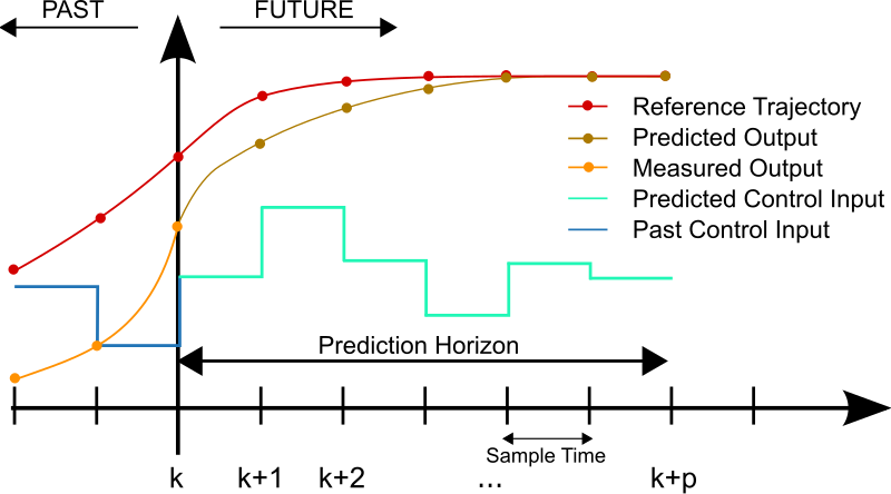
Model predictive control restates the problem of following a trajectory from a path planner to an optimization problem using a cost function, whose object is to find the optimal trajectory. In order to develop a controller that works well, a cost function needs to work within the parameters of the model and the constraints. The cost is most generally defined as the difference between where the vehicle is predicted to travel based on the model and where the vehicle is desired to go. A model predictive control implementation simulates actuator inputs, predicting the trajectory as a result of those inputs, and selecting the trajectory with the minimum cost. Once this is complete, the very first set of actuation commands is implemented. This is because the model is only an approximation, and so the trajectory calculated decreases in accuracy far into the future, meaning that the actual trajectory of the vehicle will deviate further and further from the predicted trajectory over time. Finally, the new state of the vehicle is used to feed back into the MPC, starting the process over again.

Cost functions often include features such as cross-track error (perpendicular distance from the path planner trajectory), heading error (difference between actual heading and desired heading), distance to the destination, difference between speed limit and current speed, and others. Other values can come from control inputs which cause passenger discomfort, such as absolute value of acceleration, jerk (rate of change of acceleration), absolute value of heading difference from a straight path, and change in steering.

Model predictive controllers predict concrete states several “steps” into the future; the number of steps and the time between steps are controller parameters which are chosen to maximize accuracy and allow for real-time operation of the controller.

With all of these pieces, the model predictive controller runs in a loop, with a polynomial optimizer running at each step to select the best trajectory given the initial model, the model constraints, and the cost function, which returns actuator values in sequence.

Implementation

The Model

The vehicle is modeled using a kinematic bicycle model, consisting of six elements:

• vehicle x position (x)
• vehicle y position (y)
• vehicle heading (psi)
• vehicle velocity (v)
• cross track error (cte)
• vehicle heading error (epsi)

Two actuator values are outputted by the MPC:

• steering (steer)
• throttle (accel)

The cost function for predictions includes a linear combination of seven components (each component is squared before being used, to ensure differentiability in the cost optimizer):

• cross track error
• vehicle heading error
• difference between current and target speed
• steering value (zero being steering straight; multiplied by factor of 2000)
• throttle value (zero being no acceleration nor braking)
• steering change rate (zero being no change to steering; multiplied by factor of 5)
• throttle change rate (zero being no change to throttle; multiplied by factor of 5)

The update equations for each of the states are:

• x[t+1] = x[t] + v[t] * cos(psi[t]) * dt
• y[t+1] = y[t] + v[t] * sin(psi[t]) * dt
• psi[t+1] = psi[t] + v[t] / Lf * steer[t] * dt
• v[t+1] = v[t] + accel[t] * dt
• cte[t+1] = f(x[t]) - y[t] + v[t] * sin(epsi[t]) * dt
• epsi[t+1] = psi[t] - psides[t] + v[t] * steer[t] / Lf * dt

where Lf is a simulation-based constant describing the difference between the front of the vehicle and its center of gravity.

The MPC predicts N state vectors and N-1 actuation vectors using the mathematical optimizer IPOPT. The first actuation vector is used for the each successive actuation of the vehicle (the following actuator values are not used); the state vectors are useful for debugging and visual optimization in the simulator.

Using the cost components above, the vehicle is able to drive smoothly around the simulated track at up to ~55mph without creating hazardous driving conditions.

Timestep length and Elapsed Duration

A timestep length of N = 20 and elapsed duration between timesteps of dt = 0.05 was initially chosen. However, it was found that this dt led to steering overcorrection of the vehicle, so the dt was doubled to 0.1 and N halved to 10. After that, the total length of the predicted course was found to be too short, with too many back and forth steering corrections. By increasing the N = 20, the vehicle was able to drive around the path with enough future predicted states while not predicting sharp corrections.

Polynomial fitting and MPC pre-processing

Waypoints from the simulator are received in map coordinates; before they can be used, they are converted to vehicle coordinates (using the map coordinates of the vehicle itself). These waypoints (now in vehicle coordinates) are then used to fit a 3rd degree polynomial. This polynomial is used to compute the desired location of the vehicle on the path; this allows for computing the cross track error as the distance between the desired location of the vehicle and the current location and the vehicle heading error.

Model Predictive Control with Latency

Due to a 100ms simulated actuator delay between actuator value computation and actuator implementation, any actuator values computed by the MPC are 100ms out of date by the time they arrive at the simulated vehicle. This reflects reality of true vehicle hardware. Because of this, a latency adjustment is computed which, at each actuator computation, predicts the vehicle state into the future by the latency amount. This is done simply by using the same vehicle update equations above a single time before passing the state into the MPC itself.

With these adjustments, the MPC that was implemented easily handles a 100ms latency with the simulated vehicle driving at ~55mph.

Results

The simulated vehicle drives around the track with minimal steering jerk and no sudden acceleration or deceleration. Note that the steering is much smoother than my PID controller implementation, which operates on optimizing for zero cross-track error alone.

In the video, the yellow line is a polynomial fit of the yellow line dots, which are input targets from the path planner. The green line is a polynomial fit of the green line dots, which track the optimal trajectory as determined by the MPC.

Read More