Autonomous Vehicle Technology: Sensor Fusion and Extended Kalman Filters for Object Tracking

While cameras are incredibly useful for autonomous vehicles (such as in traffic sign detection and classification), other sensors also provide invaluable data for creating a complete picture of the environment around a vehicle. Because different sensors have different capabilities, using multiple sensors simultaneously can yield a more accurate picture of the world than using one sensor alone. Sensor fusion is this technique of combining data from multiple sensors. Two frequently used non-camera-based sensor technologies used in autonomous vehicles are radar and lidar, which have different strengths and weaknesses and produce very different output data.

Radars exist in many different forms in a vehicle: for use in adaptive cruise control, blind spot warning, collision warning, collision avoidance, to name a few. Radar uses the Doppler effect to measure speed and angle to a target. Radar waves reflect off hard surfaces, but can pass through fog and rain, have a wide field of view and a long range. However, their resolution is poor compared to lidar or cameras, and they can pick up radar clutter from small objects with high reflectivity. Lidars use infrared laser beams to determine the exact location of a target. Lidar data resolution is higher than radar, but lidars cannot measure the velocity of objects, and they are more adversely affected by fog and rain.
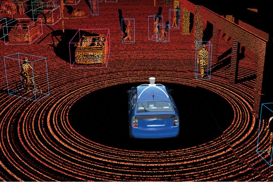
Lidar point cloud

Example of lidar point cloud

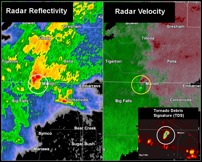
Radar map and velocity

Example of radar location and velocity data

A very popular mechanism for object tracking in autonomous vehicles is a Kalman filter. Kalman filters uses multiple imprecise measurements over time to estimate locations of objects, which is more accurate than single measurements alone. This is possible by iterating between estimating the object state and uncertainty, and updating the state and uncertainty with a new weighted measurement, with more weight being given to measurements with higher precision. This works great for linear models, but for non-linear models (such as those which involve a turning car, a bicycle, or a radar measurement), the extended Kalman filter must be used. Extended Kalman filters are considered the standard for many autonomous vehicle tracking systems.
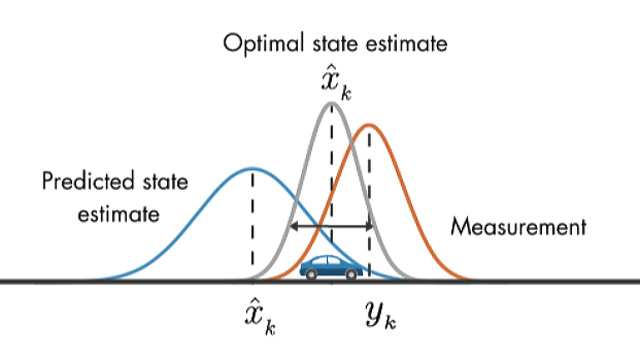
Kalman filter joint probability

I created an extended Kalman filter implementation which estimates the location and velocity of a vehicle with noisy radar and lidar measurements.

Exploring my implementation

All of the code and resources used in this project are available in my Github repository. Enjoy!

Technologies Used

  • C++
  • uWebSockets
  • Eigen

Kalman filters

Conceptually, Kalman filters work on the assumption that the actual or “true” state of the object (for instance, location and velocity) and the “true” uncertainty of the state may not be knowable. Rather, by using previous estimates about the object’s state, knowledge of how the object’s state changes (what direction it is headed and how fast), uncertainty about the movement of the vehicle, the measurement from sensors, and uncertainty about sensor measurements, an estimate of the object’s state can be computed which is more accurate than just assuming the values from raw sensor measurements.
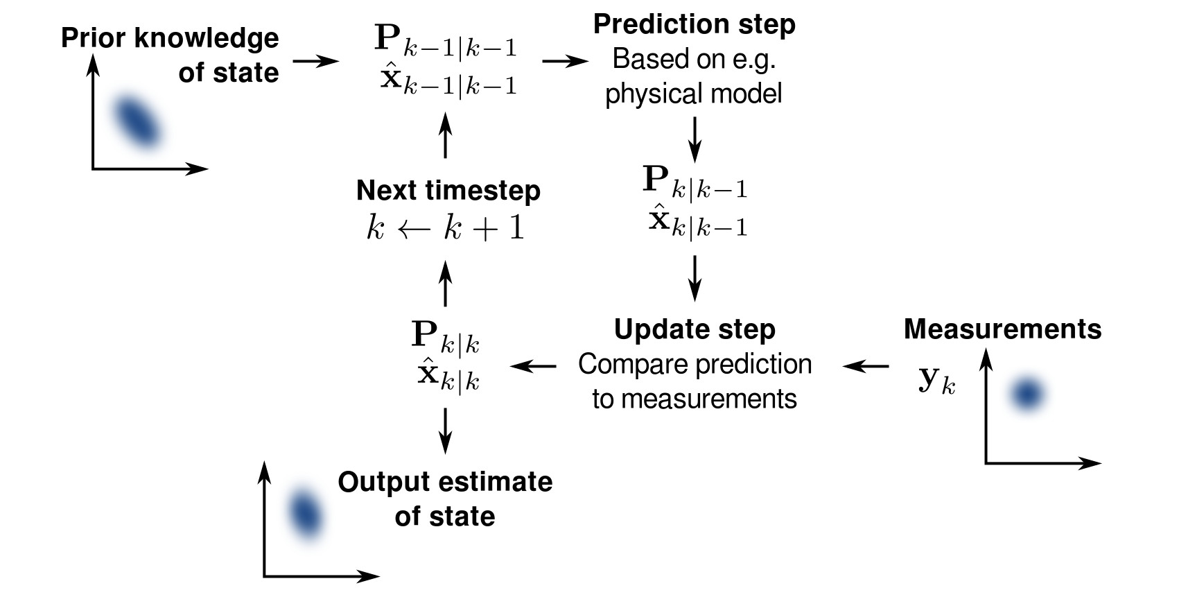
Kalman filter algorithm

With each new measurement, the “true state” of the object is “predicted”. This happens by applying knowledge about the velocity of the object as of the previous time step to the state. Because there is some uncertainty about the speed and direction that the object traveled since the last timestep (maybe the vehicle turned a corner or slowed down), we add some “noise” to the “true state”.

Next, the “true state” just predicted is modified based on the sensor measurement with an “update”. First, the sensor data is compared against belief about the true state. Next, the “Kalman filter gain”, which is the combination of the uncertainty about the predicted state and the uncertainty of the sensor measurement, is applied to the result, which updates the “true state” to the final belief of the state of the object.

Extended Kalman filters

Because the motion of the object may not be linear; for example, if it accelerates around a curve, or slows down as it exits a highway, or swerves to avoid a bicycle, the model of the object motion may be non-linear. Similarly, the mapping of the sensor observation from the true state space into the observation space may be non-linear, which is the case for radar measurements, which must map distance and angle into location and velocity. As long as the state and measurement models are differentiable functions, the basic Kalman filter can be modified to allow for these situations.

To do this, the basic Kalman filter is “extended” for non-linearity. The extended Kalman filter computations are not significantly different from the basic equations. For this example project, the state and lidar observation models will remain linear, though the radar observation model will be non-linear.

Implementation

Position estimation occurs in a main loop inside the program. First, the program waits for the next sensor measurement, either from the lidar or radar. Lidar sensor measurements contain the absolute position of the vehicle, while radar measurements contain the distance to the vehicle, angle to the vehicle, and speed of the vehicle along the angle. The measurements are passed through the sensor fusion module (which uses a Kalman filter for position estimation), then the new position estimation is compared to ground truth for performance evaluation.

The sensor fusion module encapsulates the core logic for processing a new sensor measurement and updating the estimated state (location and velocity) of the vehicle. Upon initialization, the lidar and radar measurement uncertainties are initialized (which would be provided by the sensor manufacturers), as well as the initial state uncertainty. Upon receiving a first measurement, the initial state is set to the raw measurement from the sensor (using a conversion in the case of a first measurement being from a radar). Next, the model uncertainty is computed based on the elapsed time from the previous measurement, and the “predict” step is run. Finally, the “update” step is run, with small variations depending on the measurement being from a lidar or radar (radar measurements need to be transformed from distance, angle, speed along angle to absolute world coordinates).

The Kalman filter module contains the implementations of the “predict” and “update” steps of the Kalman algorithm. The “predict” step generates a new “true state” and “true state uncertainty” using the state transition model on the current state and current state uncertainty. The “update” step operates differently depending on if running on a lidar or radar measurement. In the case of a lidar measurement, the difference between the raw measurement and the observation model applied to the predicted “true state” is used to generate a state differential. In the case of a radar measurement, the difference between the raw measurement and the “true state” transformed into radar coordinates (distance, angle, speed along angle) is used to generate a state differential. Next, the Kalman filter gain is computed which determines how the new measurement is to be weighted against the “true state”. Finally, the Kalman filter gain is applied to the state differential and added to the “true state” and “true state uncertainty” to update them to their final values.

Performance

To test the sensor fusion using the extended Kalman filter, the simulator provides raw lidar and radar measurements of the vehicle through time. Raw lidar measurements are drawn as red circles, raw radar measurements (transformed into absolute world coordinates) are drawn as blue circles with an arrow pointing in the direction of the observed angle, and sensor fusion vehicle location markers are green triangles.

Clearly, the green position estimation based on the sensor fusion tracks very closely to the vehicle location, even with imprecise measurements from the lidar and radar inputs (both by visual inspection and by the low RMSE.) Success!
Read More

Autonomous Vehicle Technology: Transfer Learning

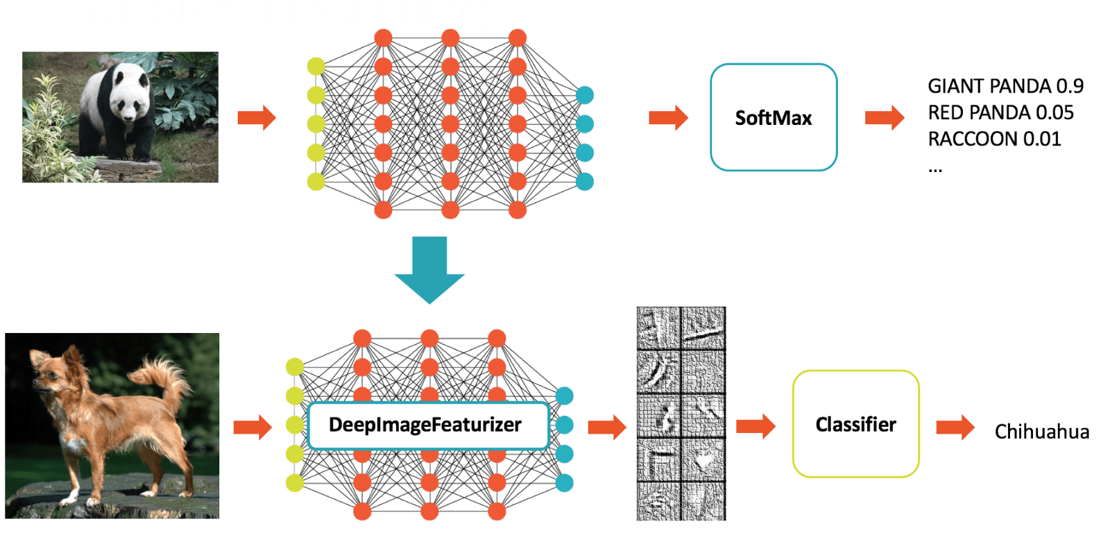
In other autonomous vehicle software stacks, I have built, trained, and operated various deep neural networks from scratch for image classification tasks, using training data I have either obtained from others or generated myself (traffic sign classification, vehicle detection and tracking, etc). However, many deep learning tasks can use pre-existing trained neural networks from some other similar task, and with some tweaks to the network itself, can significantly reduce the effort and shorten the time to production. Transfer learning is the technique of modifying and re-purposing an existing network for a new task.

Transfer LearningSome popular high-performance networks include VGG, GoogLeNet, and ResNet. Models for these networks were previously trained for days or weeks on the ImageNet dataset. The trained weights encapsulate higher-level features learned from training on thousands of classes, yet they can be adapted to be used for other datasets as well.
Exploring my implementation

I explored using transfer learning using these networks on two different datasets. All of the code and resources used are available in my Github repository. Enjoy!

Technologies Used

  • Python
  • Keras
  • Tensorflow

Example pre-trained networks

Some existing networks which can be used for new tasks using transfer learning include:

  • VGG – A great starting point for new tasks due to its simplicity and flexibility.
  • GoogLeNet – Uses an inception module to shrink the number of parameters of the model, offering improved accuracy and inference speed over VGG.
  • ResNet – Order of magnitude more layers than other networks; even better (lower error rate) than normal humans at image classification.

Transfer learning details

Depending on the size of the new dataset, and the similarity of the new dataset to the old, different approaches are typical when applying transfer learning to repurpose a pre-existing network.

Small dataset, similar to existing

  • Remove last fully connected layer from network (most other layers encode good information)
  • Add a new fully connected layer with number of classes in new dataset
  • Randomize weights of new fully connected layer, keeping other weights frozen (don’t overfit new data)
  • Train network on new data

Small dataset, different from existing

  • Remove fully connected layers and most convolutional layers towards the end of the network (most layers encode different information)
  • Add a new fully connected layer with number of classes in new dataset
  • Randomize weights of new fully connected layer, keeping other weights frozen (don’t overfit new data)
  • Train network on new data

Large dataset, similar to existing

  • Remove last fully connected layer from network (most other layers encode good information)
  • Add a new fully connected layer with number of classes in new dataset
  • Randomize weights of new fully connected layer, and initialize other layers with previous weights (don’t freeze)
  • Train network on new data

Large dataset, different from existing

  • Remove last fully connected layer from network (most other layers encode good information)
  • Add a new fully connected layer with number of classes in new dataset
  • Randomize weights on all layers
  • Train network on new data

Read More

Autonomous Vehicle Technology: Vehicle Detection and Tracking

A huge portion of the challenge in building a self-driving car is environment perception. Autonomous vehicles may use many different types of inputs to help them perceive their environment and make decisions about how to navigate. The field of computer vision includes techniques to allow a self-driving car to perceive its environment simply by looking at inputs from cameras. Cameras have a much higher spatial resolution than radar and lidar, and while raw camera images themselves are two-dimensional, their higher resolution often allows for inference of the depth of objects in a scene. Plus, cameras are much less expensive than radar and lidar sensors, giving them a huge advantage in current self-driving car perception systems. In the future, it is even possible that self-driving cars will be outfitted simply with a suite of cameras and intelligent software to interpret the images, much like a human does with its two eyes and a brain.

Detecting other vehicles and determining what path they are on are important abilities for an autonomous vehicle. They help the vehicle’s path planner to compute a safe, efficient path to follow. Vehicle detection can be performed by using object classification in an image; however, vehicles can appear anywhere in a camera’s field of view, and may look different depending on the angle and distance.

I created a software pipeline to detect and mark vehicles in a video from a front-facing vehicle camera. The following techniques are used:

  • Extract various image features (Histogram of Oriented Gradients (HOG), color transforms, binned color images) from a labeled training set of images and train a classifier.
  • Implement a sliding-window technique to search for vehicles in images using that classifier.
  • Run the pipeline on a video stream and create a heat map of recurring detections frame by frame to reject outliers and follow detected vehicles.
  • Estimate a bounding box for vehicles detected.

Exploring my implementation

All of the code and resources used in this project are available in my Github repository. Enjoy!

Technologies Used

  • Python
  • NumPy
  • OpenCV
  • SciPy
  • SKLearn

Feature Extraction

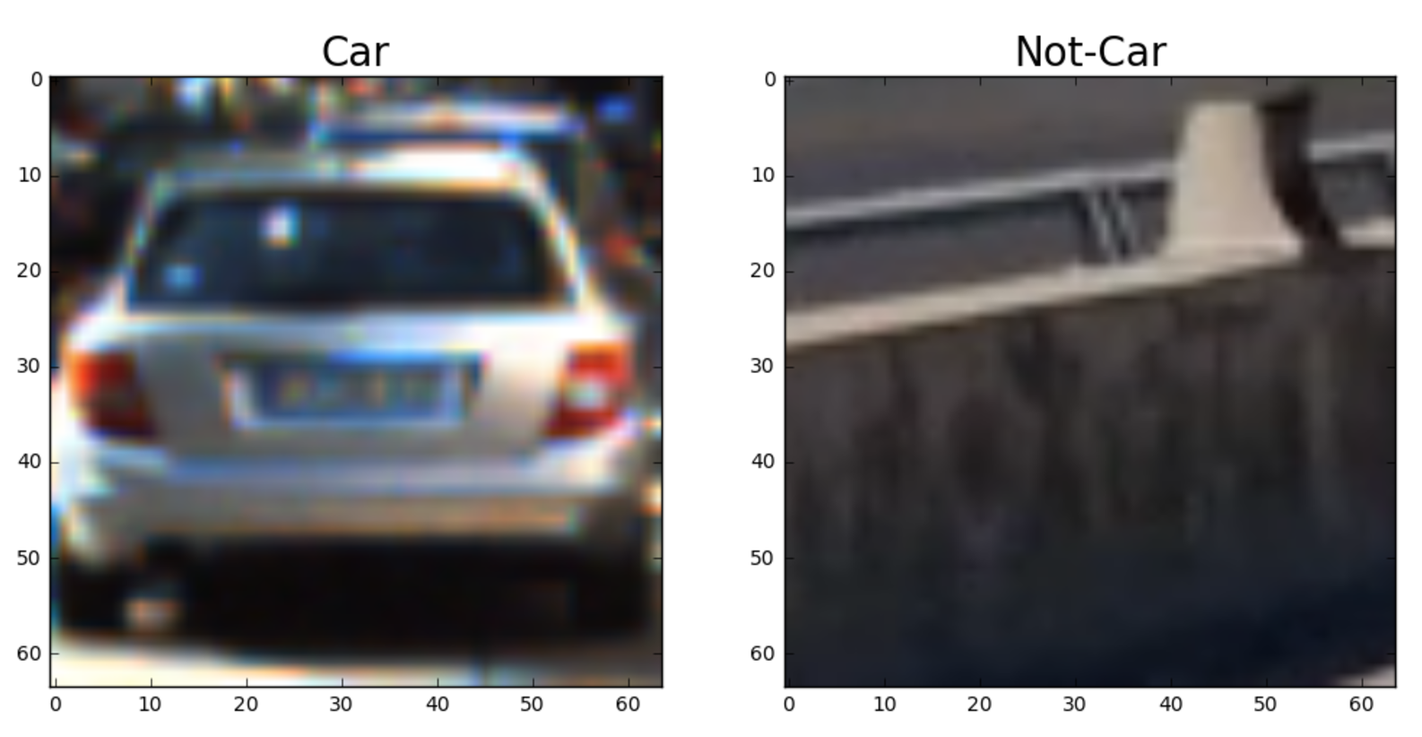
The KITTI vehicle images dataset and the extra non-vehicle images dataset is used for training data, which includes positive and negative examples of vehicles.

Here is an example of a vehicle and “not vehicle”:

Car and Not Car

Histogram of Oriented Gradients (HOG)

Because vehicles in images can appear in various shapes, sizes, and orientations, appropriate features that are robust to changes in their values is necessary. Like previous computer vision pipelines I have created, using gradients of color values in an image is often more robust than using color values themselves.

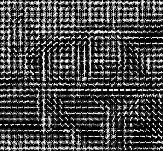
By breaking up an image into blocks of pixels, binning the gradient orientations for each pixel in the block by orientation, and selecting the orientation by the greatest bin sum (by gradient magnitudes), a single gradient can be assigned for each block. The sequence of binned gradients across the image is a histogram of oriented gradients (HOG). HOG features ignore small variations in shape while keeping the overall shape distinct.

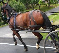
Original Image HOG representation
Horse Horse HOG

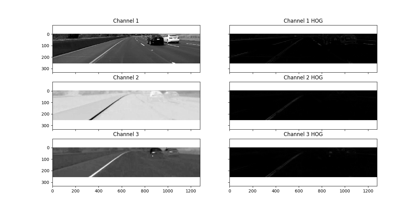
HOG features are extracted from each image in a video stream. First, the color space of the image is converted into the YCrCb color space (Luma, Blue-difference chroma and Red-difference chroma). Next, the color channels are separated and a histogram of gradient features is computed for each channel.

Here is an example of color channels and their extracted HOG features using the YCrCb color space and HOG parameters of orientations=9, pixels_per_cell=(8, 8) and cells_per_block=(2, 2):

Histogram of Oriented Gradients

HOG parameters

The general development strategy for the pipeline was to increase the accuracy of the vehicles detected in video by tuning one feature extraction parameter at a time: the feature type (HOG, spatial bins, color histogram bins), color space, and various hyperparameters for the feature type selected. While not a complete grid search of all available parameters for tuning in the feature space, the final results show reasonably good performance.

To start, HOG, color histogram, and spatial binned features were investigated separately. HOG features alone lead to the most robust classifier in terms of vehicle detection and tracking accuracy without much tuning; addition of either color histogram or spatial features greatly increases the number of false positive vehicle detections.

Different color spaces for HOG feature extraction were investigated for their performance. RGB features were quickly discarded, whose performance both in training and on sample videos is subpar to the other spaces. The YCrCb color space shows as particularly performant on both the training images and in video compared to the other color spaces investigated (YUV, LUV, HLS, HSV).

Next, various hyperparameters of the HOG transformation were optimized: number of HOG channels, number of HOG orientations, and pixels per cell (cells per block remained at 2 for all tests). In studying the classification results from both test images and video, the following parameters yield the best classification accuracy:

  • HOG channels: all
  • Number of HOG orientations: 9
  • Pixels per cell: 8

Classifier training

Next, a SVM classifier was trained for detecting vehicles in images by extracting features from a training set, scaling the feature vectors, and finally training the model.

Each vehicle and non-vehicle image had HOG features extracted. To increase the generality of the classifier, each training image was flipped on the horizontal axis in the dataset, which increased the total size of the training data to 11932 vehicle images and 10136 non-vehicle images. The relative equality of the counts of vehicle and non-vehicle images reduces the bias of any classifier towards making vehicle or non-vehicle predictions. Each one dimensional feature vector was scaled using the Scikit Learn RobustScaler, which “scales features using statistics that are robust to outliers” by using the median and interquartile range, rather than the sample mean as the StandardScaler does.

After scaling, the feature vectors were split into a training and test set, with 20% of the data used for testing.

Finally, a binary SVM classifier was trained using a linear kernel (using the SciKit Learn LinearSVC model). Results based on the training data show a 99.82% accuracy on the test data.

Upon completion of the training pipeline, I continued to experiment with other classifiers to attempt to gain better classifier performance on the test set and in videos. To do so, I tested random forests using the SciKit Learn RandomForestClassifier model, using a grid search over various parameters for optimization (using SciKit Learn GridSearchCV), and final voting of classifier based on the SciKit Learn VotingClassifier). The results show that the random forest classifier performs on-par with the support vector machine but requires more hyperparameter tuning, and so the code remains with only the LinearSVC.

Sliding Window Search

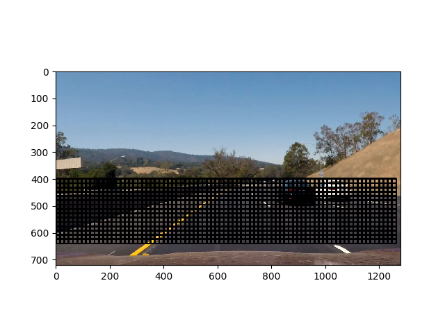
After implementing a basic classifier with reasonable performance on training data, the next step was to detect vehicles in test images and video. A “sliding window” approach is used in which a “sub-image” window (a square subset of pixels) is moved across the full image. Features are extracted from the sub-image, and the classifier determines if there is a vehicle present or not. The window slides both horizontally and vertically across the image. The window size was chosen to be 64×64 pixels, with an overlap of 75% as the detection window slides. Once all windows have been searched, the list of windows in which vehicles were detected is returned (which may include some overlap). As an early optimization to eliminate extra false positive vehicle detections, the vertical span of searching is limited from the just above the top of the horizon to just above the vehicle engine hood in the image (based on visual inspection).

As a computational optimization, the sliding window search computes HOG features for the entire image first, then the sliding windows pull in the HOG features captured by that window, and other features are computed for that window. Together with Python’s multiprocessing library, the speed improvements enabled experimentation across the various parameters in a reasonable time (~15 minutes to process a 50 second video).

Sliding Windows

In an attempt to improve vehicle detection accuracy in the project video, other window sizes were used (with multiples of 32 pixels): 64, 96, 128, 160, and 192. Overall vehicle detection accuracy decreased when using any of the other sizes. Additionally, I tried using multiple sizes at once; this caused problems further down in the vehicle detection pipeline (specifically, the bounding box smoother).

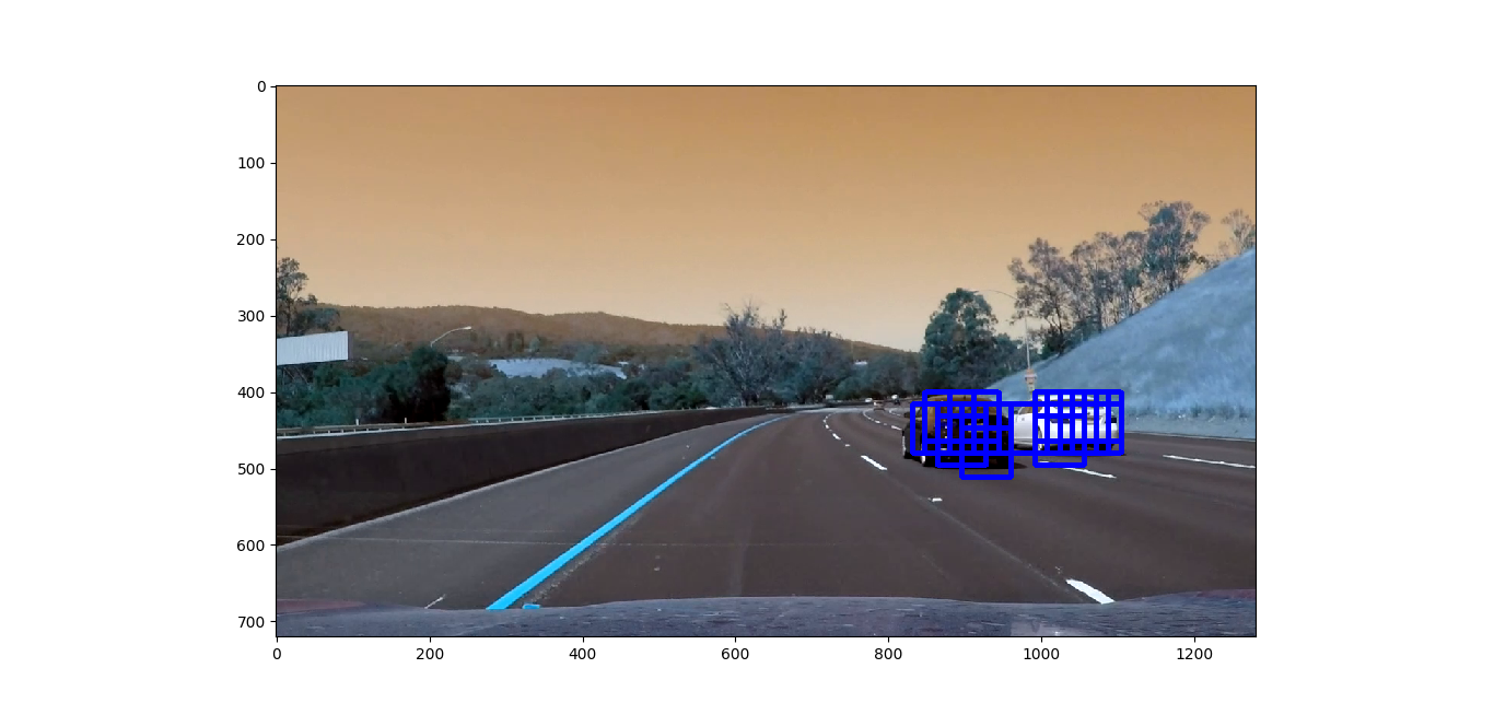
Here are some sample images showing the boxes around images which were classified as vehicles:

Vehicles Detected

Video

The pipeline generates a video stream which shows bounding boxes around the vehicles. While the bounding boxes are somewhat wobbly, and there are some false positives, the vehicles in the driving direction are identifed with relatively high accuracy. As with many machine learning classification problems, as false negatives go down, false positives go up. The heatmap threshold could be adjusted up or down to suit the end use case.

The pipeline records the positions of positive detections in each frame of the video. Positive detection regions are tracked for the current and previous four frames at each frame processing. The five total positive detections are stacked together (each pixel inside a region is one count), and then the final stacked heatmap is thresholded to identify vehicle positions (eleven counts or more per pixel being used as the threshold). I then used SciPy’s label to identify individual blobs in the heatmap. Each blob is assumed to correspond to a vehicle, and each blob is used to construct a vehicle bounding box which is drawn over the image frame.

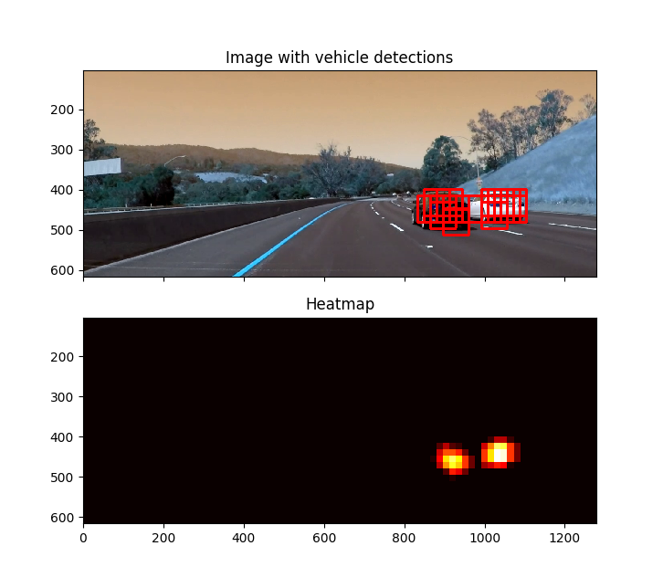
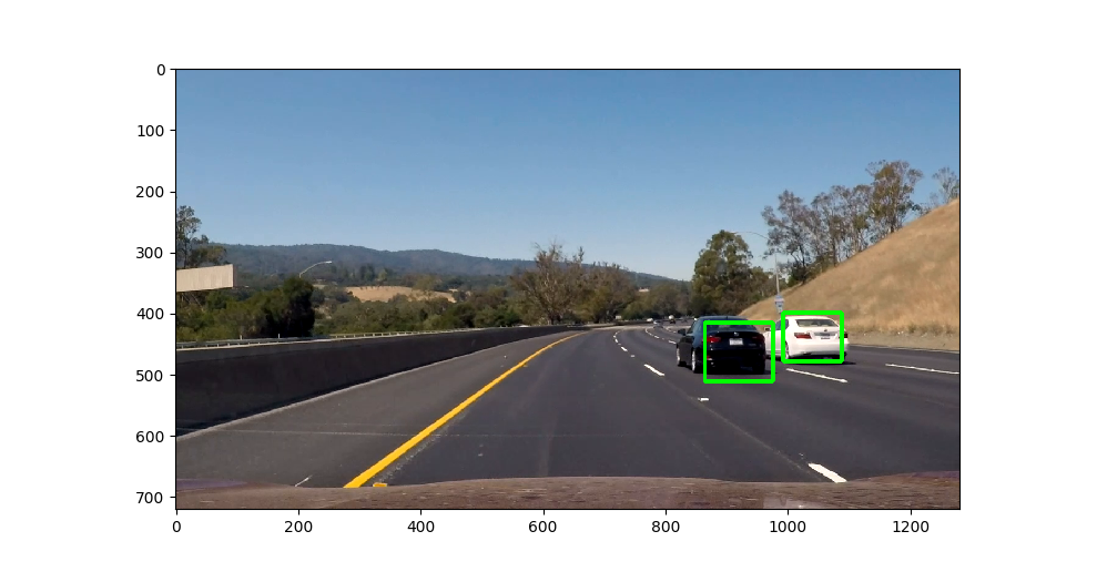
Here is an example result showing the heatmap from a series of frames of video, the result of scipy.ndimage.measurements.label() and the bounding boxes then overlaid on the last frame of video:

Here is a frame and its corresponding heatmap:

Bounding Boxes and Heatmap

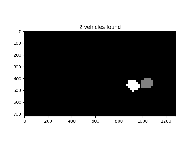
Here is the output of scipy.ndimage.measurements.label() on the integrated heatmap:

Labels Map

Here the resulting bounding boxes are drawn the image:

Final Bounding Boxes

Challenges

The most challenging part of this project was the search over the large number of parameters in the training and classification pipeline. Many different settings could be adjusted, including:

  • size and composition of the training image set
  • choice of combination of features extracted (HOG, spatial, and color histogram)
  • parameters for each type of feature extraction
  • choice of machine learning model (SVC, random forest, etc)
  • hyperparameters of machine learning model
  • sliding window size and stride
  • heatmap stack size and thresholding variable

Rather than completing an exhaustive grid search on all possibilities (which would not only have been computationally infeasible in a short period of time but also likely to overfit the training data), completing this pipeline involved iterative optimization, using a “gradient descent”-like approach to finding the next least-optimized area.

Problems in the current implementation that could be improved upon include:

  • reduction in number of false positive detections, in the form of:
    • small detections sprinkled around the video – could add more post-processing to filter out small boxes after final heat map label creation
    • a few large detections in shadow areas or with highway signs
    • not detecting the entirety of the vehicle
    • often the side of the vehicles are missed – include more training data with side images of vehicles
    • side detections can be increased by lowering the heatmap masking threshold, at the expense of more false positive vehicle detections

The pipeline would likely fail to detect in various situations, including (but not limited to):

  • vehicles other than cars – fix with more training data with other vehicles
  • nighttime detection – fix with different training data and possibly different feature extraction types / parameters
  • detection of vehicles driving perpandicular to vehicle – adjust heatmap queuing value and thresholding, possibly training data, too

Read More

Autonomous Vehicle Technology: Advanced Lane Line Detection

A huge portion of the challenge in building a self-driving car is environment perception. Autonomous vehicles may use many different types of inputs to help them perceive their environment and make decisions about how to navigate. The field of computer vision includes techniques to allow a self-driving car to perceive its environment simply by looking at inputs from cameras. Cameras have a much higher spatial resolution than radar and lidar, and while raw camera images themselves are two-dimensional, their higher resolution often allows for inference of the depth of objects in a scene. Plus, cameras are much less expensive than radar and lidar sensors, giving them a huge advantage in current self-driving car perception systems. In the future, it is even possible that self-driving cars will be outfitted simply with a suite of cameras and intelligent software to interpret the images, much like a human does with its two eyes and a brain.

When operating on roadways, correctly identifying lane lines is critical for safe vehicle operation to prevent collisions with other vehicles, road boundaries, or other objects. While GPS measurements and other object detection inputs can help to localize a vehicle with high precision according to a predefined map, following lane lines painted on the road surface is still important; real lane boundaries will always take precedence over static map boundaries.

While the previous lane line finding project allowed for identification of lane lines under ideal conditions, this lane line detection pipeline can detect lane lines the face of challenges such as curving lanes, shadows, and pavement color changes. This pipeline also computes lane curvature and the location of the vehicle relative to the center of the lane, which informs path planning and eventually control systems (steering, throttle, brake, etc).

I created a software pipeline which identifies lane boundaries in a video from a front-facing vehicle camera. The following techniques are used:

  • Compute the camera calibration matrix and distortion coefficients given a set of chessboard images.
  • Apply a distortion correction to raw images.
  • Use color transforms, gradients, etc., to create a thresholded binary image.
  • Apply a perspective transform to rectify binary image (“bird’s-eye view”)
  • Detect lane pixels and fit to find the lane boundary.
  • Determine the curvature of the lane and vehicle position with respect to center.
  • Warp the detected lane boundaries back onto the original image.
  • Output visual display of the lane boundaries and numerical estimation of lane curvature and vehicle position.

Exploring my implementation

All of the code and resources used in this project are available in my Github repository. Enjoy!

Technologies Used

  • Python
  • NumPy
  • OpenCV

Camera Calibration

Cameras do not create perfect image representations of real life. Images are often distorted, especially around the edges; edges can often get stretched or skewed. This is problematic for lane line finding as the curvature of a lane could easily be miscomputed simply due to distortion.

The qualities of the distortion for a given camera can generally be represented as five constants, collectively called the “distortion coefficients”. Once the coefficients of a given camera are computed, distortion in images produced can be reversed. To compute the distortion coefficients of a given camera, images of chessboard calibration patterns can be used. The OpenCV library has built-in methods to achieve this.

Computing the camera matrix and distortion coefficients

This method starts by preparing “object points”, which will be the (x, y, z) coordinates of the chessboard corners in the world. Here I am assuming the chessboard is fixed on the (x, y) plane at z=0, such that the object points are the same for each calibration image. Thus, objp is just a replicated array of coordinates, and objpoints will be appended with a copy of it every time I successfully detect all chessboard corners in a test image. img_points will be appended with the (x, y) pixel position of each of the corners in the image plane with each successful chessboard detection.

Next, each chessboard calibration image is processed individually. Each image is converted to grayscale, then cv2.findChessboardCorners is used to detect the corners. Corners detected are made more accurate by using cv2.cornerSubPix with a suitable search termination criteria, then the object points and image points are added for later calibration.

Finally, the image points and object points are used to compute the camera calibration and distortion coefficients using the cv2.calibrateCamera() method.

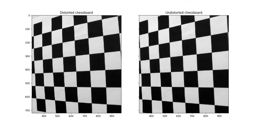
I applied this distortion correction to the test image using cv2.undistort() and obtained this result:

Chessboard distortion

Pipeline functions

Distortion correction

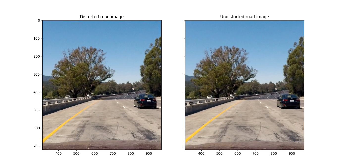
The distortion correction method correct_distortion() is used on a road image, as can be seen in this before and after image:

Undistorted Road

Binary image thresholding

Using the Sobel operator, a camera image can be transformed to reveal only strong lines that are likely to be lane lines. This has an advantage over Canny edge detection in that it ignores much of the gradient noise in an image which is not likely to be part of a lane line. Detected gradients can be filtered in both the horizontal and vertical directions using thresholds with different magnitudes to allow for much more precise detection of lane lines. Similarly, using different color channels in the gradient detection can help to increase the accuracy of lines selected.

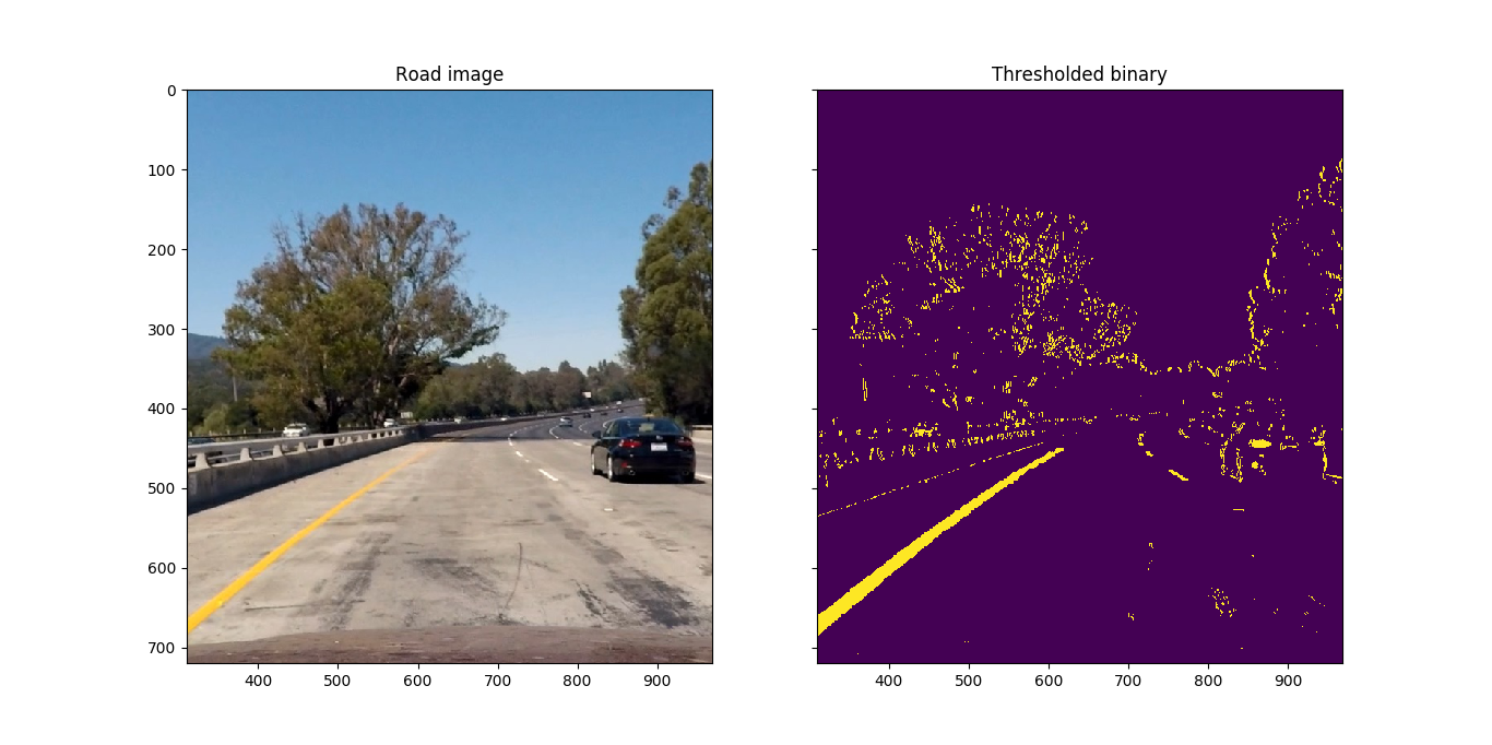
To create a thresholded binary image, I detect horizontal line segments through a Sobel x gradient computation, white lines through a identifying high signal in the L channel of the LUV color space, and yellow lines through identifying low (yellow) signal in the B channel of the LAB color space. Any pixel identified by any of the three filters contributes to the binary image.

Here is an example of an original image and a thresholded binary created from it:

Thresholded Binary image

Note that the thresholding detection picks up many other pixels that are not part of the yellow or white lane lines, though the selected pixel density in the lanes are significantly greater than the overall noise in the thresholded binary image so as to not confuse the lane line detection in a future step.

Perspective transformation

In order to determine the curvature of lane lines in an image, the lane lines need to be visualized from the top, as if from a bird’s-eye view. To do this, a perspective transform can be used to map from the front-of-vehicle view to an imaginary bird’s-eye view.

I compute a perspective transform using a hardcoded trapezoid and rectangle determined by visual inspection in the original unwarped image.

This results in the following source and destination points:

Source Destination
589, 455 300, 0
692, 455 1030, 0
1039, 676 980, 719
268, 676 250, 719

The effect of the perspective transform can be seen by viewing the pre and post-transformed images:

Warped Road

Identifying lane line pixels and lane curve extrapolation

Once raw camera images have been distortion-corrected, gradient-thresholded, and perspective-transformed, the result is ready to have lane lines identified.

I used two methods of identifying lane lines in a thresholded binary image and fitting with a polynomial. The first method identifies pixels by a naive sliding window detection algorithm; the second method identifies pixels by starting with a previous line fit. A shared code path picks the method to use, and falls back to naive sliding window search if the previous line fit does not perform.

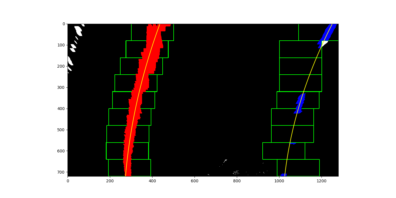
In the first method, the thresholded binary image is scanned on nine individual horizontal slices of the image. Slices start at the bottom and move up, selecting from the nearest to farthest point on the road. In each slice, a box starts at the horizontal location with the most highlighted pixels, and moves to the left or right at each step “up” the image based where most of the highlighted pixels in the box are detected, with some constraints on how far to the left or right the image can move and how big the windows are. Any pixels caught in each sliding window are used for a 2nd degree polynomial curve fit. This method is performed twice for each image, to attempt to capture both left and right lanes.

Here is an example of a thresholded binary with sliding windows and polynomial fit lines drawn over:

Polynomial Lane Line Fit

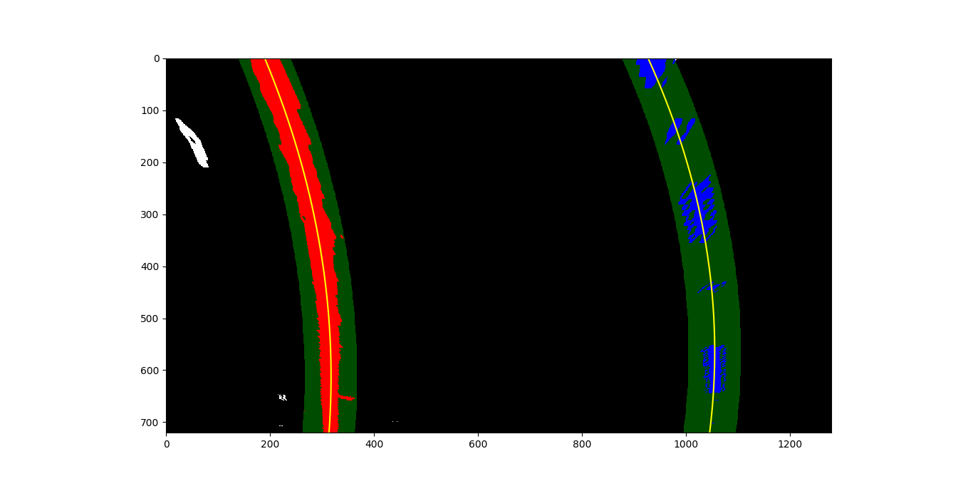
In the second method, two previous polynomial fit lines are used (likely taken from a previous frame of video) to generate a “channel” around the line with a given margin. Only highlighted pixels in the “channel” around the line are used for the next fit line. This method can ignore more noise than first method; this comes in particularly useful in areas of shadow or many yellow or white areas in the image that are not lane lines. This method can also fail if no pixels are detected in the “channel” around the previous line.

Here is an example of a thresholded binary with previous fit channels and polynomial fit lines drawn over:

Polynomial Lane Line Fit Limited

Radius of curvature / vehicle position calculation

In this detection pipeline, radius of curvature computation is intertwined with curve and lane line detection smoothing.

In the first method, the radius of curvature is determined by computing the radius of curvature equation (straightforward algebra).

In the second method (which provides a small degree of curvature and lane smoothing from video frame to frame), the raw lane lines detected in the previous step are combined with the lane lines found in the previous ten frames of video. Lane lines whose curvatures are more than 1.5 standard deviations from the median are ignored, and the remaining curvatures are averaged. The lane lines with the curvature closest to the average are selected for both drawing onto the final image, as well as for the chosen curvature.

Lane detection overlay

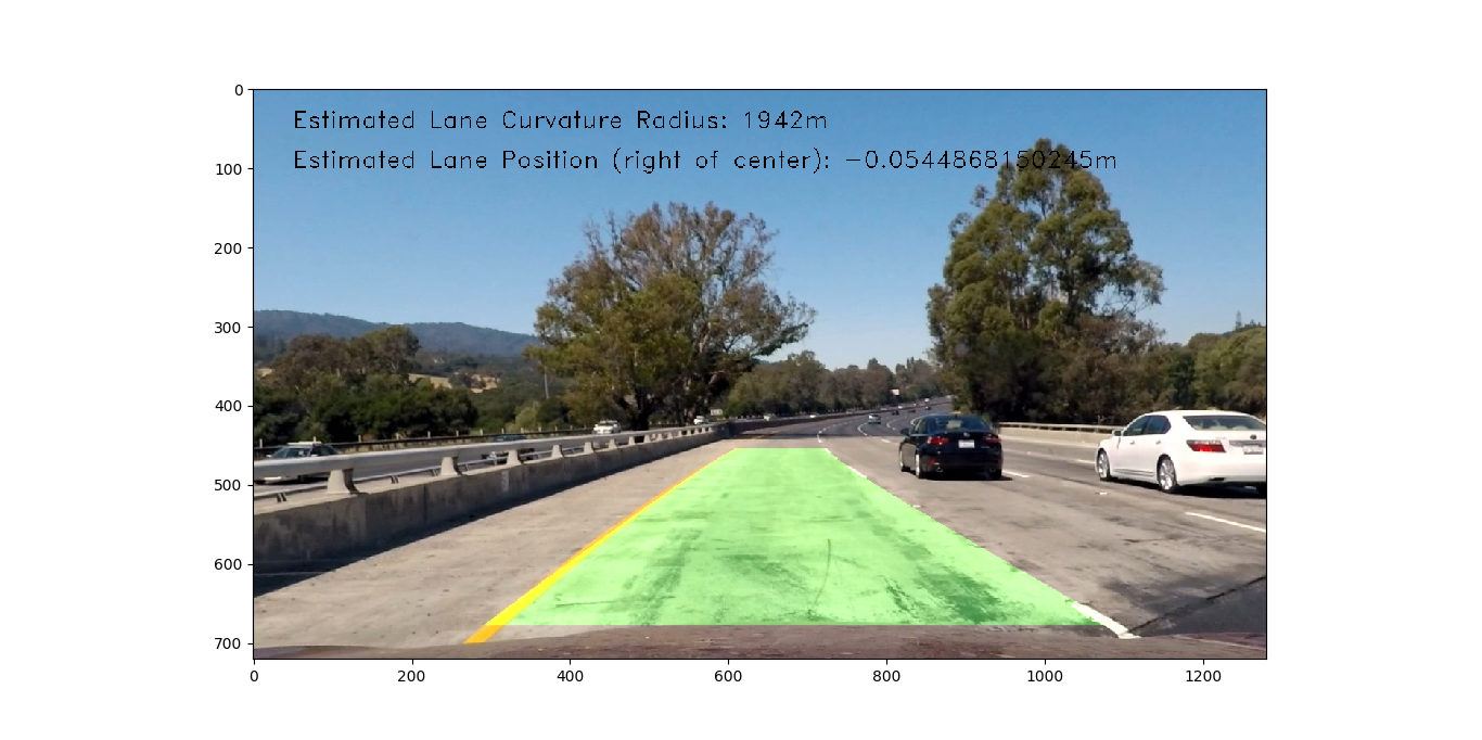
After the lane line is chosen by the smoothing algorithm above, the lane line pixels are drawn back onto the image, resulting in this:

Final Lane Detection

Final video output

The lane detection algorithm was run on three videos:

Standard Video

Lane finding is quite robust, having some slight wobbles when the vehicle bounces across road surface changes and when shadows appear in the roadway

More difficult video

Lane finding is useful throughout the entire video, though the lane detection algorithm selects a shadow edge rather than the yellow lane line for a portion of the video

Most difficult video

Lane finding is primitive, staying with the lane for only a small portion of the time.

Problems / Issues

One of the biggest issues in the pipeline is non-lane line pixel detection in the thresholded binary image creator. Because of the simple nature of having channel thresholding in color spaces be the determiner of what pixels are likely part of lane lines, groups of errant pixels (“noise”) were occassionally added to the thresholded binary image which were not part of the lane lines.

Another big issue is that the lane line detection algorithms are not sufficiently robust to ignore this noise at all times. The naive sliding window algorithm, in particular, is sensitive to blocks of noise in the vicinity of actual lane lines, which shows up in the project videos in locations where large shadows intersect with lane lines. The polynomial fit-restricted lane line detection algorithm can ignore most of this noise, but if the lane line detection sways from the true line, recovery to the true line may take many frames.

Fixing these problems required tuning of the thresholded binary pixel detection and a substantial investment in lane line detection smoothing and outlier detection. However, because generally bad input data often leads to bad output (“garbage in, garbage out”), more time should be spent on improving noise reduction in the thresholded binary image before further tuning downstream.

Likely failure scenarios

It is already clear in the videos presented that the pipeline has occasional failures when lane lines cannot be clearly detected due to shadows cast. Other likely problem triggers include:

  • Lanes not being painted clearly / faded / missing
  • Vehicle decides to drive offroad and ignore lanes
  • Vehicle drives in an area without yellow or while lanes

Future improvements

Future modifications to increase the robustness of the lane detection might include:

  • Improving upon naive line detection algorithm to help eliminate effect of noise
  • Look for other lane colors
  • Use multiple steps in lane line pixel detection to use detectors with highest specificity first, then fall back to those with lower specificity if lane lines cannot be determine from initial thresholded binary
  • Improving upon smoothing algorithm
  • Use concept of “keyframing” from video compression technology to periodically revert back to naive line detection, even if polynomial fit line detection has detected a line, in case it is tracking a bad line segment

Read More