Autonomous Vehicle Technology: Localization using Particle Filters

In order to drive safely, autonomous vehicles on public roads need to know where they are in the world. Tasks easy for humans, such as staying in driving lanes at all times, would be impossible for an autonomous vehicle to perform without highly accurate vehicle location information. Determining the vehicle’s location in the world is called localization. One popular and well-known localization system is the global positioning system (GPS), which can provide rough localization; it often has accuracy of one to three meters, but the accuracy can decrease to upwards of fifty meters with poor line off sight to the sky or other interference. Unfortunately, this is not accurate enough for an autonomous vehicle; a localization accuracy of under ten centimeters is considered the upper limit for safe driving.

Like the techniques involved in object tracking using extended and unscented Kalman filters, localization techniques are often probabilistic. The unscented Kalman filter is flexible enough for many object tracking applications; however, when even higher accuracy is required for vehicle localization, another technique can be used: a particle filter.


Exploring my implementation

All of the code and resources used in this project are available in my Github repository. Enjoy!

Technologies Used

  • C++
  • uWebSocketIO

Particle Filters

Particle filters are similar to unscented Kalman filters in that they update the state of an object (for example, the location and orientation) by transforming a set of points through a function to predict a future state, given noisy and partial observations of the world. However, unlike unscented Kalman filters, particle filters may choose points to transform at random, rather than from a Gaussian distribution. This eliminates the need to assume a static state motion or measurement model. The number of points required for a particle filter to obtain the same level of accuracy as an unscented Kalman filter is generally higher, which makes a particle filter more computationally complex and memory intensive. Additionally, there is a choice to be made regarding the number of particles included in the filter (the time complexity of computing the algorithm is linear in the number of particles). However, particle filters do converge to the true state of the object being predicted as number of particles increases, unlike unscented Kalman filters, which have no such convergence properties.

Particle filter steps

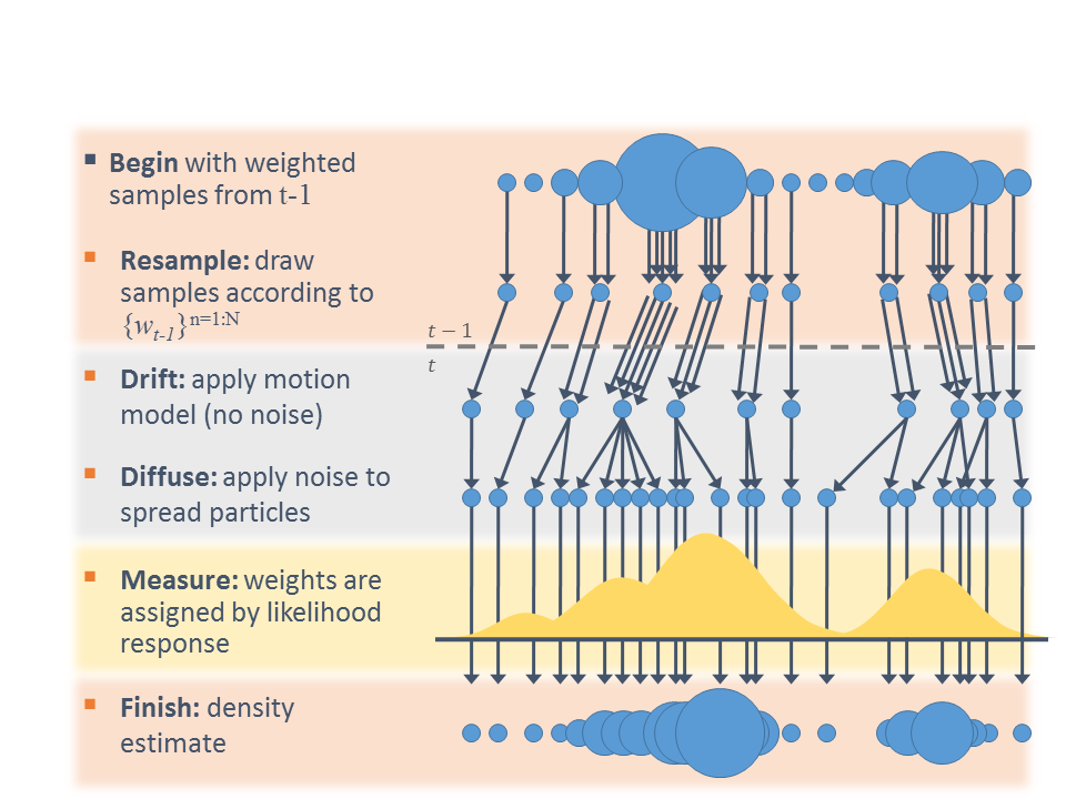
In a particle filter, the points, or “particles”, are chosen to represent concrete guesses as to the actual state being predicted. At each time step, particles are randomly sampled from the state space. The probability of a particle being chosen is proportional to the probablility of it being the correct state, given the sensor measurements seen so far. The update step in a particle filter can be seen as selecting the most likely hypotheses among the set of guessed states; as more sensor measurements become available, those more likely to be true are kept, while those less likely are removed.

Particle filters for localization

When used for localization, particle filters become a particularly effective technique. Because they can approximate non-parametric functions, they perform better in many non-linear model environments, including situations with multiple possible localization positions. For example, when using a Kalman filter (extended or unscented), a vehicle driving down a road with many similar lampposts may decide that it is next to a lamppost, but may have trouble determining which lamppost it is next to.

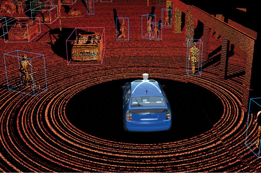
In using a particle filter for localization, data from onboard sensors (such as radar and lidar) can be used to measure distances to static objects (trees, poles, walls), which may involve sensor fusion. With a pre-loaded map which has trusted coordinates of these fixed objects, a particle filter matches observations of objects in the world against those in the map, and then determines where the vehicle is in the map space. To start, particles may initially be chosen at random from all locations, with no assumptions about where the vehicle is. However, in practice, some sort of one-time hint about the general location from GPS may be provided. At each time step, the algorithm uses its previous belief about vehicle location, the current vehicle control values, and sensor measurements, and outputs a new belief about the vehicle location.

The algorithm runs by updating the current set of particles (possible locations) according to the vehicle control command, simulating motion of all of the particles. For instance, if the vehicle is travelling forward, all particles move forward. If the vehicle turns to the right, all of the particles turn to the right. Because the result of a control does not always complete as expected, some amount of noise is added to the particle movement to simulate this uncertainty. Each particle is then considered to be the possible location of the vehicle, and the probability that the location is the true location of the vehicle given the current sensor measurements is computed. Those probabilities are used as weights to randomly select new particles from the previous particle list. Because of this, particles which are consistent with sensor measurements are more likely to be chosen (and may even be chosen more than once!), and particles which are inconsisent with the measurements are less likely to be chosen. However, to prevent convergence on an incorrect location (if the vehicle is stationary, for instance), extra uniformly sampled particles can be added.

With every iteration of the particle filter algorithm, the selected particles converge to the true location of the vehicle, which makes intuitive sense: as the vehicle senses more of its environment, it should be expected to become increasingly sure of its position.

Localization maze

Implementation

The localization algorithm exists as a loop, where new sensor measurements and control commands are read. On the first sensor measurement, the particle filter is initialized with that measurement; on subsequent measurements, the particle filter is run to predict the new location of the vehicle. Next, the particles have their weights updated using observations from sensors and known map landmarks, then particles are resampled. Finally, the particle with the highest weight is chosen as the new location of the vehicle.

Inside the particle filter, the initialization step creates 100 particles, locates them all at the first measurement, and then adjusts each particle randomly according to the sensor measurement uncertainty distribution. During prediction, each particle’s next location is predicted by moving it according to the velocity and turn rate from most recent vehicle control command.

To update the weights for each particle based on the sensor observations of landmarks, the landmarks nearest the particle are chosen. Next, each observation is paired with its closest true landmark. Finally, the particle’s weight is set to the product of the distance between each true landmark and its closest observation.

Particle resampling occurs according to the particles weights, which is a standard sampling with replacement approach.

Performance

To test the localization using the particle filter, the simulator provides sensor measurements of fixed objects in the world. These are plotted in the simulator as black crosses with circles around them. Green lines drawn between the vehicle and the circles indicate fixed objects which are being tracked.

The jitter between the vehicle (true location) and the grey circle (predicted location) is kept to a relative minimum over time, even during accelerations, decelerations, and turns. This indicates that the filter does a relatively good job at localization.

Read More

Autonomous Vehicle Technology: Sensor Fusion and Unscented Kalman Filters for Object Tracking

While cameras are incredibly useful for autonomous vehicles (such as in traffic sign detection and classification), other sensors also provide invaluable data for creating a complete picture of the environment around a vehicle. Because different sensors have different capabilities, using multiple sensors simultaneously can yield a more accurate picture of the world than using one sensor alone. Sensor fusion is this technique of combining data from multiple sensors. Two frequently used non-camera-based sensor technologies used in autonomous vehicles are radar and lidar, which have different strengths and weaknesses and produce very different output data.

Radars exist in many different forms in a vehicle: for use in adaptive cruise control, blind spot warning, collision warning, collision avoidance, to name a few. Radar uses the Doppler effect to measure speed and angle to a target. Radar waves reflect off hard surfaces, but can pass through fog and rain, have a wide field of view and a long range. However, their resolution is poor compared to lidar or cameras, and they can pick up radar clutter from small objects with high reflectivity. Lidars use infrared laser beams to determine the exact location of a target. Lidar data resolution is higher than radar, but lidars cannot measure the velocity of objects, and they are more adversely affected by fog and rain.

Lidar point cloud

Example of lidar point cloud

Radar map and velocity

Example of radar location and velocity data

A very popular mechanism for object tracking in autonomous vehicles is a Kalman filter. Kalman filters uses multiple imprecise measurements over time to estimate locations of objects, which is more accurate than single measurements alone. This is possible by iterating between estimating the object state and uncertainty, and updating the state and uncertainty with a new weighted measurement, with more weight being given to measurements with higher precision. This works great for linear models, but for non-linear models (such as those which involve a turning car, a bicycle, or a radar measurement), the extended Kalman filter must be used. Extended Kalman filters are considered the standard for many autonomous vehicle tracking systems.

Unfortunately, when the models are very non-linear, the extended Kalman filter can yield very poor performance. As a remedy, the unscented Kalman filter can be used.

Kalman filter joint probability

Exploring my implementation

All of the code and resources used in this project are available in my Github repository. Enjoy!

Technologies Used

  • C++
  • uWebSockets

Kalman filters

Conceptually, Kalman filters work on the assumption that the actual or “true” state of the object (for instance, location and velocity) and the “true” uncertainty of the state may not be knowable. Rather, by using previous estimates about the object’s state, knowledge of how the object’s state changes (what direction it is headed and how fast), uncertainty about the movement of the vehicle, the measurement from sensors, and uncertainty about sensor measurements, an estimate of the object’s state can be computed which is more accurate than just assuming the values from raw sensor measurements.

Kalman filter algorithm

With each new measurement, the “true state” of the object is “predicted”. This happens by applying knowledge about the velocity of the object as of the previous time step to the state. Because there is some uncertainty about the speed and direction that the object traveled since the last timestep (maybe the vehicle turned a corner or slowed down), we add some “noise” to the “true state”.

Next, the “true state” just predicted is modified based on the sensor measurement with an “update”. First, the sensor data is compared against belief about the true state. Next, the “Kalman filter gain”, which is the combination of the uncertainty about the predicted state and the uncertainty of the sensor measurement, is applied to the result, which updates the “true state” to the final belief of the state of the object.

Unscented Kalman filters

Because the motion of the object may not be linear; for example, if it accelerates around a curve, or slows down as it exits a highway, or swerves to avoid a bicycle, the model of the object motion may be non-linear. Similarly, the mapping of the sensor observation from the true state space into the observation space may be non-linear, which is the case for radar measurements, which must map distance and angle into location and velocity. The extended Kalman filter can often be used here when the non-linear motion or observation models are easily differentiable and can be approximated by a linear functions.

However, in some cases the motion or observation models are either not easily differentiable or cannot be easily approximated by linear functions. For example, many motion models use non-constant velocity; often they include both straight lines and turns. Even if these functions could be differentiated properly, the probability distributions of the uncertainty in the models might not be normally distributed after a “predict” or “update” step, which breaks the Kalman filter assumptions. To avoid this problem, using an unscented Kalman filter can be used, which involves transforming point samples from a Gaussian distribution through the non-linear models to approximate the final probability distribution. This has two main advantages:

* the sample points often approximate the probability distribution of the non-linear functions better than a linear model does

* a Jacobian matrix is not necessary to compute

In order to preserve the “normal” nature of the motion and observation probability distributions, the unscented Kalman filter uses the “unscented transformation” to map a set of points through the motion and observation models. To do this, a group of “sigma points” are selected which represent the original state probability distribution. Once transformed by the non-linear model, the mean and per-dimensional standard deviations of the transformed points are computed, which yields a useful approximation of the real mean and standard deviation of the non-linear model.

Other than using sigma points to represent the motion and observation model probability functions, the unscented Kalman filter flow is similar to that of the extended Kalman filter, including a measurement-model independent “predict” step, followed by a measurement-model dependent “update” step.

Implementation

Position estimation occurs in a main loop inside the program. First, the program waits for the next sensor measurement, either from the lidar or radar. Lidar sensor measurements contain the absolute position of the vehicle, while radar measurements contain the distance to the vehicle, angle to the vehicle, and speed of the vehicle along the angle. The measurements are passed through the sensor fusion module (which uses a Kalman filter for position estimation), then the new position estimation is compared to ground truth for performance evaluation.

The unscented Kalman filter module encapsulates the core logic for processing a new sensor measurement and updating the estimated state (location and velocity) of the vehicle. Upon initialization, the lidar and radar measurement uncertainties are initialized (which would be provided by the sensor manufacturers), as well as the motion model uncertainty. Upon receiving a first measurement, the initial state is set to the raw measurement from the sensor (using a conversion in the case of the first measurement being from a radar). Next, the “predict” and “update” steps are run.

The “predict” step has three main functions:

  • generating sigma points
  • predicting the sigma points through the motion model transform
  • predicting the new state mean and covariances

There are two different “update” implementations; one for radar and one for lidar. Both implementations must first transform the predicted sigma points into the measurement space, then update the predicted state based on the transformed measurements.

Performance

To test the sensor fusion using the unscented Kalman filter, the simulator provides raw lidar and radar measurements of the vehicle through time. Raw lidar measurements are drawn as red circles, raw radar measurements (transformed into absolute world coordinates) are drawn as blue circles with an arrow pointing in the direction of the observed angle, and sensor fusion vehicle location markers are green triangles.

Clearly, the green position estimation based on the sensor fusion tracks very closely to the vehicle location, even with imprecise measurements from the lidar and radar inputs (both by visual inspection and by the low RMSE.)

Additionally, by comparison with the extended Kalman filter on the same input dataset, it is clear that the error in the estimated positions from the unscented Kalman filter are lower than that of the extended Kalman filter:

Extended Unscented Reduction in Error
PX 0.0974 0.0756 22%
PY 0.0855 0.0849 1%
VX 0.4517 0.3530 22%
PY 0.4404 0.2428 45%

Read More

Autonomous Vehicle Technology: Sensor Fusion and Extended Kalman Filters for Object Tracking

While cameras are incredibly useful for autonomous vehicles (such as in traffic sign detection and classification), other sensors also provide invaluable data for creating a complete picture of the environment around a vehicle. Because different sensors have different capabilities, using multiple sensors simultaneously can yield a more accurate picture of the world than using one sensor alone. Sensor fusion is this technique of combining data from multiple sensors. Two frequently used non-camera-based sensor technologies used in autonomous vehicles are radar and lidar, which have different strengths and weaknesses and produce very different output data.

Radars exist in many different forms in a vehicle: for use in adaptive cruise control, blind spot warning, collision warning, collision avoidance, to name a few. Radar uses the Doppler effect to measure speed and angle to a target. Radar waves reflect off hard surfaces, but can pass through fog and rain, have a wide field of view and a long range. However, their resolution is poor compared to lidar or cameras, and they can pick up radar clutter from small objects with high reflectivity. Lidars use infrared laser beams to determine the exact location of a target. Lidar data resolution is higher than radar, but lidars cannot measure the velocity of objects, and they are more adversely affected by fog and rain.

Lidar point cloud

Example of lidar point cloud

Radar map and velocity

Example of radar location and velocity data

A very popular mechanism for object tracking in autonomous vehicles is a Kalman filter. Kalman filters uses multiple imprecise measurements over time to estimate locations of objects, which is more accurate than single measurements alone. This is possible by iterating between estimating the object state and uncertainty, and updating the state and uncertainty with a new weighted measurement, with more weight being given to measurements with higher precision. This works great for linear models, but for non-linear models (such as those which involve a turning car, a bicycle, or a radar measurement), the extended Kalman filter must be used. Extended Kalman filters are considered the standard for many autonomous vehicle tracking systems.

Kalman filter joint probability

I created an extended Kalman filter implementation which estimates the location and velocity of a vehicle with noisy radar and lidar measurements.

Exploring my implementation

All of the code and resources used in this project are available in my Github repository. Enjoy!

Technologies Used

  • C++
  • uWebSockets
  • Eigen

Kalman filters

Conceptually, Kalman filters work on the assumption that the actual or “true” state of the object (for instance, location and velocity) and the “true” uncertainty of the state may not be knowable. Rather, by using previous estimates about the object’s state, knowledge of how the object’s state changes (what direction it is headed and how fast), uncertainty about the movement of the vehicle, the measurement from sensors, and uncertainty about sensor measurements, an estimate of the object’s state can be computed which is more accurate than just assuming the values from raw sensor measurements.

Kalman filter algorithm

With each new measurement, the “true state” of the object is “predicted”. This happens by applying knowledge about the velocity of the object as of the previous time step to the state. Because there is some uncertainty about the speed and direction that the object traveled since the last timestep (maybe the vehicle turned a corner or slowed down), we add some “noise” to the “true state”.

Next, the “true state” just predicted is modified based on the sensor measurement with an “update”. First, the sensor data is compared against belief about the true state. Next, the “Kalman filter gain”, which is the combination of the uncertainty about the predicted state and the uncertainty of the sensor measurement, is applied to the result, which updates the “true state” to the final belief of the state of the object.

Extended Kalman filters

Because the motion of the object may not be linear; for example, if it accelerates around a curve, or slows down as it exits a highway, or swerves to avoid a bicycle, the model of the object motion may be non-linear. Similarly, the mapping of the sensor observation from the true state space into the observation space may be non-linear, which is the case for radar measurements, which must map distance and angle into location and velocity. As long as the state and measurement models are differentiable functions, the basic Kalman filter can be modified to allow for these situations.

To do this, the basic Kalman filter is “extended” for non-linearity. The extended Kalman filter computations are not significantly different from the basic equations. For this example project, the state and lidar observation models will remain linear, though the radar observation model will be non-linear.

Implementation

Position estimation occurs in a main loop inside the program. First, the program waits for the next sensor measurement, either from the lidar or radar. Lidar sensor measurements contain the absolute position of the vehicle, while radar measurements contain the distance to the vehicle, angle to the vehicle, and speed of the vehicle along the angle. The measurements are passed through the sensor fusion module (which uses a Kalman filter for position estimation), then the new position estimation is compared to ground truth for performance evaluation.

The sensor fusion module encapsulates the core logic for processing a new sensor measurement and updating the estimated state (location and velocity) of the vehicle. Upon initialization, the lidar and radar measurement uncertainties are initialized (which would be provided by the sensor manufacturers), as well as the initial state uncertainty. Upon receiving a first measurement, the initial state is set to the raw measurement from the sensor (using a conversion in the case of a first measurement being from a radar). Next, the model uncertainty is computed based on the elapsed time from the previous measurement, and the “predict” step is run. Finally, the “update” step is run, with small variations depending on the measurement being from a lidar or radar (radar measurements need to be transformed from distance, angle, speed along angle to absolute world coordinates).

The Kalman filter module contains the implementations of the “predict” and “update” steps of the Kalman algorithm. The “predict” step generates a new “true state” and “true state uncertainty” using the state transition model on the current state and current state uncertainty. The “update” step operates differently depending on if running on a lidar or radar measurement. In the case of a lidar measurement, the difference between the raw measurement and the observation model applied to the predicted “true state” is used to generate a state differential. In the case of a radar measurement, the difference between the raw measurement and the “true state” transformed into radar coordinates (distance, angle, speed along angle) is used to generate a state differential. Next, the Kalman filter gain is computed which determines how the new measurement is to be weighted against the “true state”. Finally, the Kalman filter gain is applied to the state differential and added to the “true state” and “true state uncertainty” to update them to their final values.

Performance

To test the sensor fusion using the extended Kalman filter, the simulator provides raw lidar and radar measurements of the vehicle through time. Raw lidar measurements are drawn as red circles, raw radar measurements (transformed into absolute world coordinates) are drawn as blue circles with an arrow pointing in the direction of the observed angle, and sensor fusion vehicle location markers are green triangles.

Clearly, the green position estimation based on the sensor fusion tracks very closely to the vehicle location, even with imprecise measurements from the lidar and radar inputs (both by visual inspection and by the low RMSE.) Success!

Read More

Autonomous Vehicle Technology: Transfer Learning

In other autonomous vehicle software stacks, I have built, trained, and operated various deep neural networks from scratch for image classification tasks, using training data I have either obtained from others or generated myself (traffic sign classification, vehicle detection and tracking, etc). However, many deep learning tasks can use pre-existing trained neural networks from some other similar task, and with some tweaks to the network itself, can significantly reduce the effort and shorten the time to production. Transfer learning is the technique of modifying and re-purposing an existing network for a new task.

Transfer LearningSome popular high-performance networks include VGG, GoogLeNet, and ResNet. Models for these networks were previously trained for days or weeks on the ImageNet dataset. The trained weights encapsulate higher-level features learned from training on thousands of classes, yet they can be adapted to be used for other datasets as well.

Exploring my implementation

I explored using transfer learning using these networks on two different datasets. All of the code and resources used are available in my Github repository. Enjoy!

Technologies Used

  • Python
  • Keras
  • Tensorflow

Example pre-trained networks

Some existing networks which can be used for new tasks using transfer learning include:

  • VGG – A great starting point for new tasks due to its simplicity and flexibility.
  • GoogLeNet – Uses an inception module to shrink the number of parameters of the model, offering improved accuracy and inference speed over VGG.
  • ResNet – Order of magnitude more layers than other networks; even better (lower error rate) than normal humans at image classification.

Transfer learning details

Depending on the size of the new dataset, and the similarity of the new dataset to the old, different approaches are typical when applying transfer learning to repurpose a pre-existing network.

Small dataset, similar to existing

  • Remove last fully connected layer from network (most other layers encode good information)
  • Add a new fully connected layer with number of classes in new dataset
  • Randomize weights of new fully connected layer, keeping other weights frozen (don’t overfit new data)
  • Train network on new data

Small dataset, different from existing

  • Remove fully connected layers and most convolutional layers towards the end of the network (most layers encode different information)
  • Add a new fully connected layer with number of classes in new dataset
  • Randomize weights of new fully connected layer, keeping other weights frozen (don’t overfit new data)
  • Train network on new data

Large dataset, similar to existing

  • Remove last fully connected layer from network (most other layers encode good information)
  • Add a new fully connected layer with number of classes in new dataset
  • Randomize weights of new fully connected layer, and initialize other layers with previous weights (don’t freeze)
  • Train network on new data

Large dataset, different from existing

  • Remove last fully connected layer from network (most other layers encode good information)
  • Add a new fully connected layer with number of classes in new dataset
  • Randomize weights on all layers
  • Train network on new data

Read More