Autonomous Vehicle Technology: Advanced Lane Line Detection

A huge portion of the challenge in building a self-driving car is environment perception. Autonomous vehicles may use many different types of inputs to help them perceive their environment and make decisions about how to navigate. The field of computer vision includes techniques to allow a self-driving car to perceive its environment simply by looking at inputs from cameras. Cameras have a much higher spatial resolution than radar and lidar, and while raw camera images themselves are two-dimensional, their higher resolution often allows for inference of the depth of objects in a scene. Plus, cameras are much less expensive than radar and lidar sensors, giving them a huge advantage in current self-driving car perception systems. In the future, it is even possible that self-driving cars will be outfitted simply with a suite of cameras and intelligent software to interpret the images, much like a human does with its two eyes and a brain.

When operating on roadways, correctly identifying lane lines is critical for safe vehicle operation to prevent collisions with other vehicles, road boundaries, or other objects. While GPS measurements and other object detection inputs can help to localize a vehicle with high precision according to a predefined map, following lane lines painted on the road surface is still important; real lane boundaries will always take precedence over static map boundaries.

While the previous lane line finding project allowed for identification of lane lines under ideal conditions, this lane line detection pipeline can detect lane lines the face of challenges such as curving lanes, shadows, and pavement color changes. This pipeline also computes lane curvature and the location of the vehicle relative to the center of the lane, which informs path planning and eventually control systems (steering, throttle, brake, etc).

I created a software pipeline which identifies lane boundaries in a video from a front-facing vehicle camera. The following techniques are used:

  • Compute the camera calibration matrix and distortion coefficients given a set of chessboard images.
  • Apply a distortion correction to raw images.
  • Use color transforms, gradients, etc., to create a thresholded binary image.
  • Apply a perspective transform to rectify binary image (“bird’s-eye view”)
  • Detect lane pixels and fit to find the lane boundary.
  • Determine the curvature of the lane and vehicle position with respect to center.
  • Warp the detected lane boundaries back onto the original image.
  • Output visual display of the lane boundaries and numerical estimation of lane curvature and vehicle position.

Exploring my implementation

All of the code and resources used in this project are available in my Github repository. Enjoy!

Technologies Used

  • Python
  • NumPy
  • OpenCV

Camera Calibration

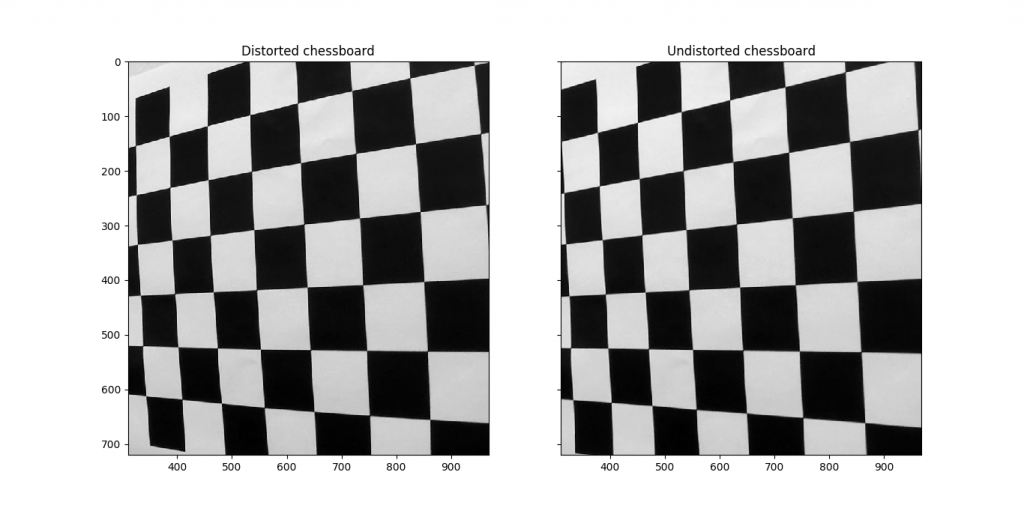
Cameras do not create perfect image representations of real life. Images are often distorted, especially around the edges; edges can often get stretched or skewed. This is problematic for lane line finding as the curvature of a lane could easily be miscomputed simply due to distortion.

The qualities of the distortion for a given camera can generally be represented as five constants, collectively called the “distortion coefficients”. Once the coefficients of a given camera are computed, distortion in images produced can be reversed. To compute the distortion coefficients of a given camera, images of chessboard calibration patterns can be used. The OpenCV library has built-in methods to achieve this.

Computing the camera matrix and distortion coefficients

This method starts by preparing “object points”, which will be the (x, y, z) coordinates of the chessboard corners in the world. Here I am assuming the chessboard is fixed on the (x, y) plane at z=0, such that the object points are the same for each calibration image. Thus, objp is just a replicated array of coordinates, and objpoints will be appended with a copy of it every time I successfully detect all chessboard corners in a test image. img_points will be appended with the (x, y) pixel position of each of the corners in the image plane with each successful chessboard detection.

Next, each chessboard calibration image is processed individually. Each image is converted to grayscale, then cv2.findChessboardCorners is used to detect the corners. Corners detected are made more accurate by using cv2.cornerSubPix with a suitable search termination criteria, then the object points and image points are added for later calibration.

Finally, the image points and object points are used to compute the camera calibration and distortion coefficients using the cv2.calibrateCamera() method.

I applied this distortion correction to the test image using cv2.undistort() and obtained this result:

Chessboard distortion

Pipeline functions

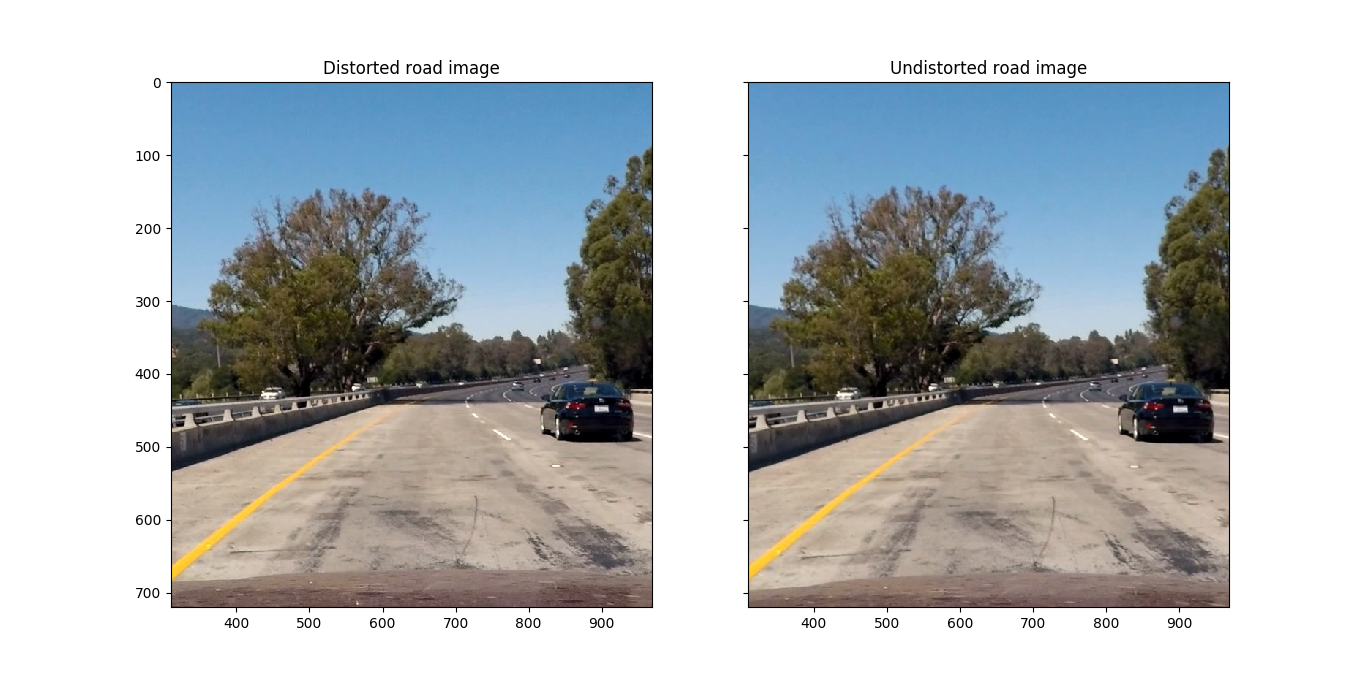
Distortion correction

The distortion correction method correct_distortion() is used on a road image, as can be seen in this before and after image:

Undistorted Road

Binary image thresholding

Using the Sobel operator, a camera image can be transformed to reveal only strong lines that are likely to be lane lines. This has an advantage over Canny edge detection in that it ignores much of the gradient noise in an image which is not likely to be part of a lane line. Detected gradients can be filtered in both the horizontal and vertical directions using thresholds with different magnitudes to allow for much more precise detection of lane lines. Similarly, using different color channels in the gradient detection can help to increase the accuracy of lines selected.

To create a thresholded binary image, I detect horizontal line segments through a Sobel x gradient computation, white lines through a identifying high signal in the L channel of the LUV color space, and yellow lines through identifying low (yellow) signal in the B channel of the LAB color space. Any pixel identified by any of the three filters contributes to the binary image.

Here is an example of an original image and a thresholded binary created from it:

Thresholded Binary image

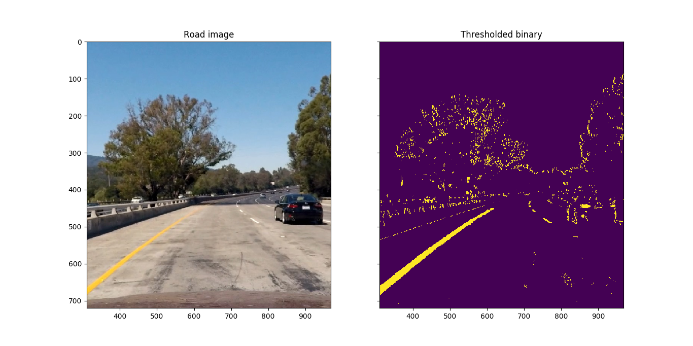
Note that the thresholding detection picks up many other pixels that are not part of the yellow or white lane lines, though the selected pixel density in the lanes are significantly greater than the overall noise in the thresholded binary image so as to not confuse the lane line detection in a future step.

Perspective transformation

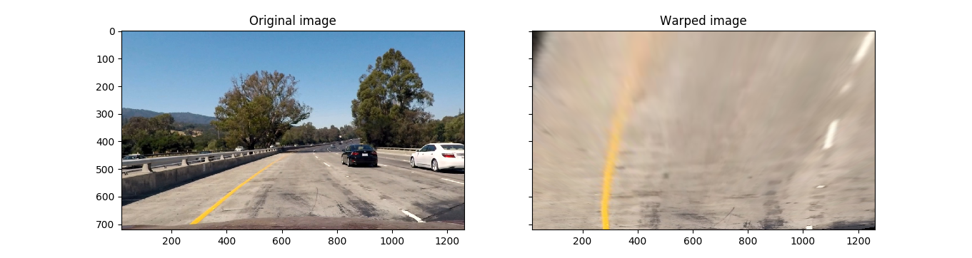
In order to determine the curvature of lane lines in an image, the lane lines need to be visualized from the top, as if from a bird’s-eye view. To do this, a perspective transform can be used to map from the front-of-vehicle view to an imaginary bird’s-eye view.

I compute a perspective transform using a hardcoded trapezoid and rectangle determined by visual inspection in the original unwarped image.

This results in the following source and destination points:

Source Destination
589, 455 300, 0
692, 455 1030, 0
1039, 676 980, 719
268, 676 250, 719

The effect of the perspective transform can be seen by viewing the pre and post-transformed images:

Warped Road

Identifying lane line pixels and lane curve extrapolation

Once raw camera images have been distortion-corrected, gradient-thresholded, and perspective-transformed, the result is ready to have lane lines identified.

I used two methods of identifying lane lines in a thresholded binary image and fitting with a polynomial. The first method identifies pixels by a naive sliding window detection algorithm; the second method identifies pixels by starting with a previous line fit. A shared code path picks the method to use, and falls back to naive sliding window search if the previous line fit does not perform.

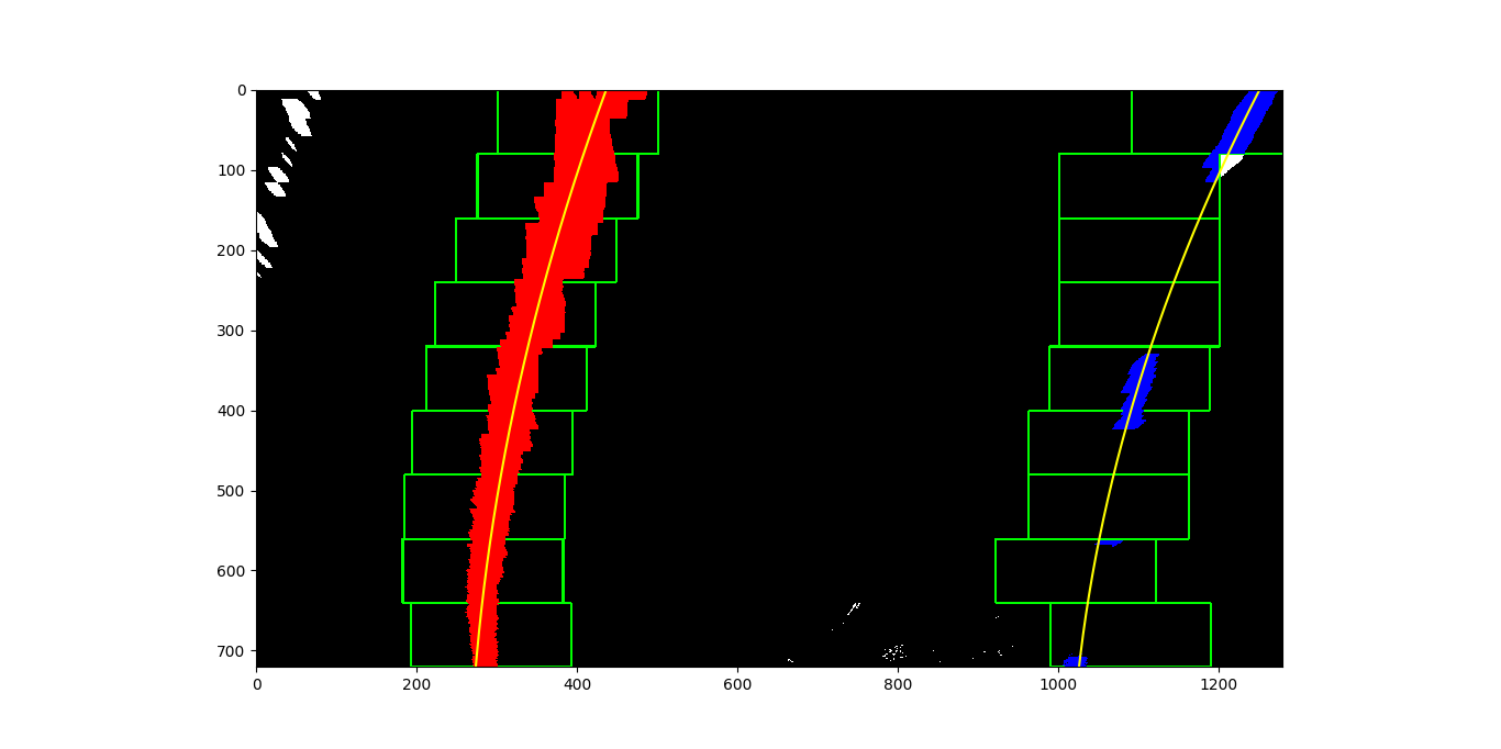
In the first method, the thresholded binary image is scanned on nine individual horizontal slices of the image. Slices start at the bottom and move up, selecting from the nearest to farthest point on the road. In each slice, a box starts at the horizontal location with the most highlighted pixels, and moves to the left or right at each step “up” the image based where most of the highlighted pixels in the box are detected, with some constraints on how far to the left or right the image can move and how big the windows are. Any pixels caught in each sliding window are used for a 2nd degree polynomial curve fit. This method is performed twice for each image, to attempt to capture both left and right lanes.

Here is an example of a thresholded binary with sliding windows and polynomial fit lines drawn over:

Polynomial Lane Line Fit

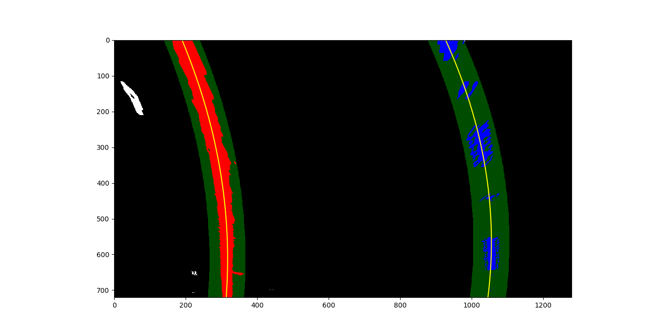
In the second method, two previous polynomial fit lines are used (likely taken from a previous frame of video) to generate a “channel” around the line with a given margin. Only highlighted pixels in the “channel” around the line are used for the next fit line. This method can ignore more noise than first method; this comes in particularly useful in areas of shadow or many yellow or white areas in the image that are not lane lines. This method can also fail if no pixels are detected in the “channel” around the previous line.

Here is an example of a thresholded binary with previous fit channels and polynomial fit lines drawn over:

Polynomial Lane Line Fit Limited

Radius of curvature / vehicle position calculation

In this detection pipeline, radius of curvature computation is intertwined with curve and lane line detection smoothing.

In the first method, the radius of curvature is determined by computing the radius of curvature equation (straightforward algebra).

In the second method (which provides a small degree of curvature and lane smoothing from video frame to frame), the raw lane lines detected in the previous step are combined with the lane lines found in the previous ten frames of video. Lane lines whose curvatures are more than 1.5 standard deviations from the median are ignored, and the remaining curvatures are averaged. The lane lines with the curvature closest to the average are selected for both drawing onto the final image, as well as for the chosen curvature.

Lane detection overlay

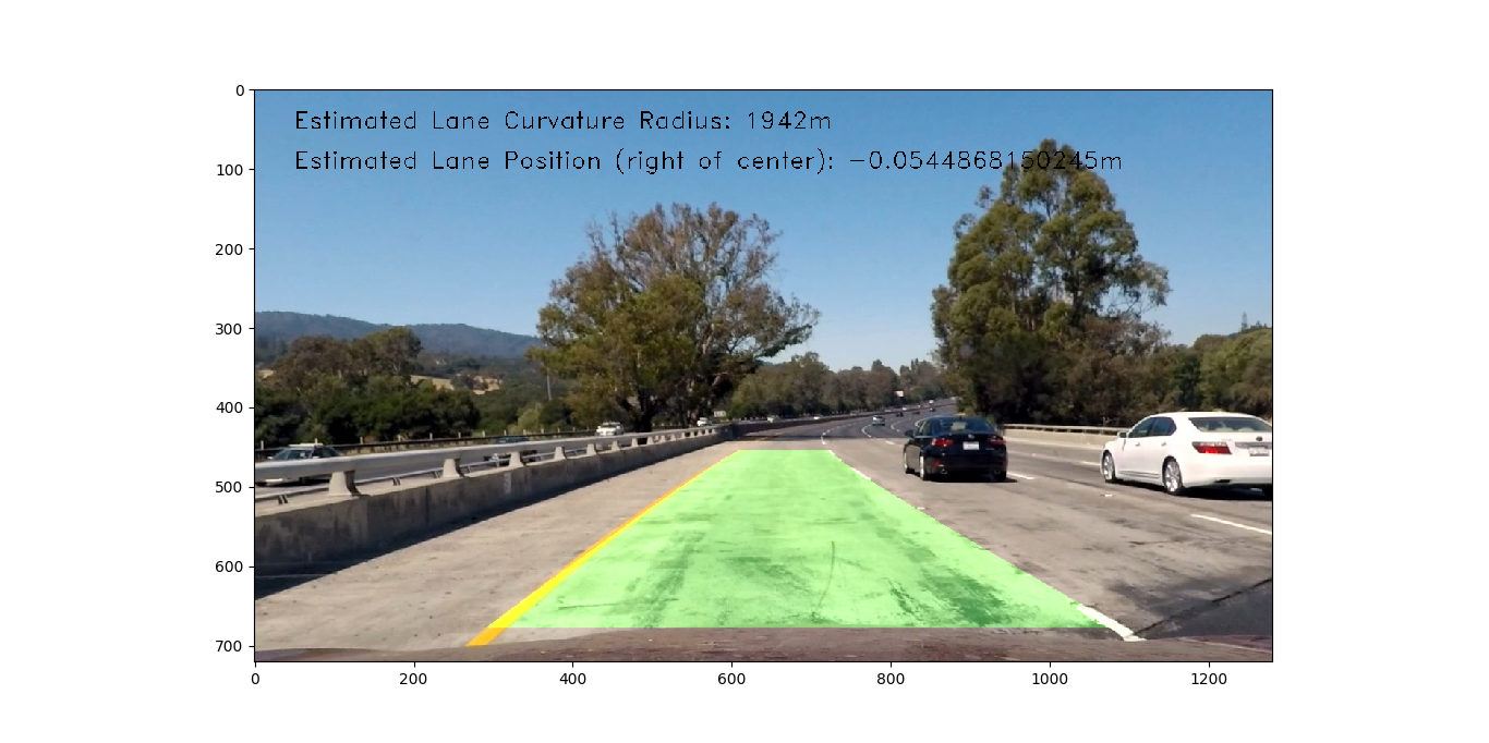
After the lane line is chosen by the smoothing algorithm above, the lane line pixels are drawn back onto the image, resulting in this:

Final Lane Detection

Final video output

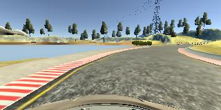
The lane detection algorithm was run on three videos:

Standard Video

Lane finding is quite robust, having some slight wobbles when the vehicle bounces across road surface changes and when shadows appear in the roadway

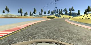
More difficult video

Lane finding is useful throughout the entire video, though the lane detection algorithm selects a shadow edge rather than the yellow lane line for a portion of the video

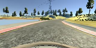
Most difficult video

Lane finding is primitive, staying with the lane for only a small portion of the time.

Problems / Issues

One of the biggest issues in the pipeline is non-lane line pixel detection in the thresholded binary image creator. Because of the simple nature of having channel thresholding in color spaces be the determiner of what pixels are likely part of lane lines, groups of errant pixels (“noise”) were occassionally added to the thresholded binary image which were not part of the lane lines.

Another big issue is that the lane line detection algorithms are not sufficiently robust to ignore this noise at all times. The naive sliding window algorithm, in particular, is sensitive to blocks of noise in the vicinity of actual lane lines, which shows up in the project videos in locations where large shadows intersect with lane lines. The polynomial fit-restricted lane line detection algorithm can ignore most of this noise, but if the lane line detection sways from the true line, recovery to the true line may take many frames.

Fixing these problems required tuning of the thresholded binary pixel detection and a substantial investment in lane line detection smoothing and outlier detection. However, because generally bad input data often leads to bad output (“garbage in, garbage out”), more time should be spent on improving noise reduction in the thresholded binary image before further tuning downstream.

Likely failure scenarios

It is already clear in the videos presented that the pipeline has occasional failures when lane lines cannot be clearly detected due to shadows cast. Other likely problem triggers include:

  • Lanes not being painted clearly / faded / missing
  • Vehicle decides to drive offroad and ignore lanes
  • Vehicle drives in an area without yellow or while lanes

Future improvements

Future modifications to increase the robustness of the lane detection might include:

  • Improving upon naive line detection algorithm to help eliminate effect of noise
  • Look for other lane colors
  • Use multiple steps in lane line pixel detection to use detectors with highest specificity first, then fall back to those with lower specificity if lane lines cannot be determine from initial thresholded binary
  • Improving upon smoothing algorithm
  • Use concept of “keyframing” from video compression technology to periodically revert back to naive line detection, even if polynomial fit line detection has detected a line, in case it is tracking a bad line segment

Read More

Autonomous Vehicle Technology: Behavioral Cloning

Humans learn through observing behavior from others. They watch and emulate the behaviors they see, making adjustments to their own actions along the way, given feedback. The same technique can be used in autonomous vehicles to model driving behavior based on direct observation of human driving. This technique is known as behavioral cloning.

I created a software suite to implement behavioral cloning for generating autonomous vehicle steering control. Using a front-facing video stream of safe driving paired with steering angles as training data, I built a convolutional neural network and trained it (using Keras) to clone driving behavior. Given a set of three front-facing camera images (front, left, and right), the model outputs a target steering wheel command.

The following techniques are used in this system:

  • Use a vehicle simulator to generate and collect data of good driving behavior
  • Build and train a convolution neural network in Keras that predicts steering angles from images
  • Train and validate the model with a training and validation set
  • Test that the model successfully drives around track one without leaving the road

Exploring my implementation

All of the code and resources used in this project are available in my Github repository. Enjoy!

Technologies used

  • Python
  • Keras
  • NumPy
  • OpenCV
  • Scikit-learn

Training a model

python model.py

Will train a model to drive the vehicle in the simulator.

Driving the simulated vehicle using the model

Once the model has been saved, it can be used with drive.py using this command:

python drive.py model.h5

Note: There is a known local system setting issue with replacing “,” with “.” when using drive.py. When this happens it can make predicted steering values clipped to max/min values. If this occurs, a known fix for this is to set the environment variable LANG to en_US.utf8.

Saving a video of the simulated vehicle using the model

python drive.py model.h5 run1

python video.py run1

Will create a video of the simulated vehicle driving with the model. The output will be a file called run1.mp4.

Optionally, one can specify the FPS (frames per second) of the video:

python video.py run1 --fps 48

Will run the video at 48 FPS. The default FPS is 60.

Model Architecture

The overall strategy for building the software’s neural network was to start with a well-known and high-performance network, and tune it for this particular steering angle prediction task.

This system includes a convolutional neural network model similar to the published NVidia architecture used for their self-driving car efforts, given that this system is attempting to solve the exact same problem (steering angle command prediction) and NVidia’s network is state of the art. This network inputs 160×320 RGB images from multiple camera angles at the front of a vehicle and outputs a single steering wheel angle command. One convolutional and one fully connected layer were removed from the NVidia architecture to reduce memory processing costs during training.

Before the convolutional layers of the model, a cropping layer removes the top (including sky) and bottom (including car image), to reduce noise in training. An additional layer normalizes the data points to have zero mean and a low standard deviation.

In between the convolutional layers, RELU activations are included to introduce non-linearity, max pooling to reduce overfitting and computatational complexity, and 50% dropout during training (also to reduce overfitting).

In between the fully-connected layers of the model, RELU activations are also introduced.

The input images are cropped to remove the top 50 and bottom 20 pixels to reduce noise in the image which are likely to be uncorrelated with steering commands. Each pixel color value in the image is then normalized to [-0.5,0.5].

Neural Network Layers

The network includes:

  • input cropping and normalization layers
  • four convolutional layers
  • three 5×5 filters with 24, 36, and 48 depth
  • one 3×3 filter with 64 depth
  • a maximum pooling layer with 2×2 pooling
  • three fully-connected layers with 100, 50, and 10 outputs
  • a final steering angle output layer
Layer Description
Input 160x320x3 RGB color image
Cropping 50 pixel top, 20 pixel bottom crop
Normalization [0,255] -> [-0.5,0.5]
Convolution 5×5 1×1 stride, valid padding, output depth 24
RELU
Max pooling 2×2 stride
Convolution 5×5 1×1 stride, valid padding, output depth 36
RELU
Max pooling 2×2 stride
Convolution 5×5 1×1 stride, valid padding, output depth 48
RELU
Max pooling 2×2 stride
Convolution 3×3 1×1 stride, valid padding, output depth 64
RELU
Max pooling 2×2 stride
Flattening 2d image -> 1d pixel values
Fully connected 100 output neurons
RELU
Dropout 50% keep fraction
Fully connected 50 output neurons
RELU
Dropout 50% keep fraction
Fully connected 10 output neurons
Output Output – 1 steering angle command

Model training

Dataset

A vehicle simulator was used to collect a dataset of images to feed into the network. Training data was chosen to keep the vehicle driving on the road, which provided center, left, and right images taken from different points on the front of the vehicle. This data includes multiple laps using center lane driving. Here is an example image of center lane driving:

Simulated center lane driving

I then recorded the vehicle recovering from the left side and right sides of the road back to center so that the vehicle would learn to correct major driving errors when the vehicle is about to run off the road. These images show what a recovery looks like starting from the left side:

Left recovery 1

Left recovery 2

Left recovery 3

To augment the data set, I also flipped images and angles during training to further generalize the model. After the collection process, I had 8253 data image frames, each including center, left, and right images for a total of 24759.

Training

During training, the entire image data set is shuffled, with 80% of the images being used for training and 20% used for validation. I configured the Keras training to use an early stopping condition based on knee-finding using the validation loss, with a patience of 2 epochs. Also, an Adam optimizer is used so that manually training the learning rate is not necessary.

Video Result

The simulated vehicle drives around the entire track without any unsafe driving behavior; in only one spot did the simulated vehicle get close to running of the track on a curve (but did not leave the driving surface, pop up on legdes, or roll over any unsafe surfaces).

Read More

Autonomous Vehicle Technology: Traffic Sign Classification

A huge portion of the challenge in building a self-driving car is environment perception. Autonomous vehicles may use many different types of inputs to help them perceive their environment and make decisions about how to navigate. The field of computer vision includes techniques to allow a self-driving car to perceive its environment simply by looking at inputs from cameras. Cameras have a much higher spatial resolution than radar and lidar, and while raw camera images themselves are two-dimensional, their higher resolution often allows for inference of the depth of objects in a scene. Plus, cameras are much less expensive than radar and lidar sensors, giving them a huge advantage in current self-driving car perception systems. In the future, it is even possible that self-driving cars will be outfitted simply with a suite of cameras and intelligent software to interpret the images, much like a human does with its two eyes and a brain.

When operating on roadways, autonomous vehicles need to be able to identify traffic signs in order to determine what actions, if any, the vehicle must take. For example, a yield sign warns drivers that other vehicle traffic will soon enter the vehicle’s path, and that those other vehicles should be given the right of way. Without a robust mechanism to quickly and correctly identify the meaning of traffic signs, autonomous vehicles would get into trouble with hazardous road conditions and with other vehicles.

I created a software pipeline containing a convolutional neural networks to classify traffic signs. The pipeline trains and validates a neural network model so it can classify traffic sign images using the German Traffic Sign Dataset. Additionally, a study of model performance on images of unseen German traffic signs from the internet is included.

Exploring my implementation

All of the code and resources used in this project are available in my Github repository. Enjoy!

Technologies used

  • Python
  • Jupyter
  • NumPy
  • OpenCV
  • SkLearn
  • Tensorflow

Data Set Summary & Exploration

The pandas library is used to calculate summary statistics of the traffic signs data set:

  • The size of training set is 34799
  • The size of the validation set is 4410
  • The size of test set is 12630
  • The shape of a traffic sign image is (32, 32, 3)
  • The number of unique classes/labels in the data set is 43

The following charts show the distribution of the instance classes in the training, validation, and test datasets.

Note how in all of the datasets, some of the classes (1-5,7-10,12-13,38) have a much higher representation in each dataset than others. This may cause bias in the predictions generated by the classifier itself; additional classification robustness could be added by adding extra instances of the classes which are under-represented.

Training data instance class distribution

Traffic Sign Classifier Training Class Distribution

Validation data instance class distribution

Traffic Sign Classifier Validation Data Class Distribution

Test data instance class distribution

Traffic Sign Classifier Test Data Class Distribution

Design and Testing of model architecture

Image data preprocessing

As a first step, all images are converted to grayscale to reduce the dimensionality of the problem that the classifier needs to learn. Given the small number of training examples (< 100k), the extra dimensionality in representing colors might overwhelm the optimizer and it would not fit a robust model. Grayscale was also used in my previous lane finding project, and given the success of finding detail in a low-resolution grayscale image similar success here is expected.

Here is an example of a traffic sign image before and after grayscaling.

Grayscale Traffic Signs

As a last step, image data is normalized to have mean zero and low standard deviation for each pixel value, to allow the learning optimizer to have an easier time converging on a lower overall classification loss.

Even though a class imbalance exists in the training data set, the training set is not augmented with more data to study the bias of the final classifier (which would be revealed during the validation step).

Final neural network architecture

The neural network model consists of the following layers:

Layer Description
Input 32x32x1 grayscale image
Convolution 5×5 1×1 stride, valid padding, outputs 28x28x6
RELU
Max pooling 2×2 stride, outputs 14x14x6
Convolution 5×5 1×1 stride, valid padding, outputs 10x10x16
RELU
Max pooling 2×2 stride, outputs 5x5x16
Fully connected 400 input neurons, 400 output neurons
RELU
Dropout 50% keep fraction
Fully connected 400 input neurons, 400 output neurons
RELU
Dropout 50% keep fraction
Fully connected 400 input neurons, 43 output neurons
Output – Softmax Output

Model training

To train the model, the following techniques are used:

  • Use of a loss function which reduces the mean of the softmax cross entropy between the output and the validation labels
  • Penalization of the loss using L2 regularization for each of the five weight groups in the network (2x convolution weight groups and 3x fully connected layer weight groups), scaled to 1% of the L2 norm
  • Optimization of the weights and biases for each of the layers using the Adam algorithm, with an initial learning rate of 0.0005 (the Adam optimizer dynamically adjusts the effective learning rate over time)
  • Mini-batching of 128 training instances looped with a maximum of 200 epochs of training and weight optimization until the accuracy is above 93.5%. 93.7% is hit after 16 epochs, at which point the training loop completes.

Improving validation set accuracy

The final model results are:

  • training set accuracy of 97.0%
  • validation set accuracy of 93.7%
  • test set accuracy of 90.5%

The neural network began with the classic LeNet-5 image classification architecture, being a canonical and well-understood image classification neural net architecture for grayscale image classification. This seemed like an obvious starting point to classify small (32×32 pixel) grayscale images with a limited set of output classes (43).

Modifications are added based on the Alexnet image processing architecture, as it is also well-understood and makes significant performance improvements on LeNet. Further modifications include using 50% dropout layers after every fully connected layer to prevent overfitting on training data, making the fully connected layers not reduce dimensionality (input and output dimensions are the same until the final output layer), and starting with initial positive values for layer bias terms rather than zero (since ReLU is used as an activation function, it is desired to prevent more connections to drop out than absolutely necessary).

Training set accuracy shows that the model is fitting to the training data well; perhaps too well, as a 97% accuracy is quite high. Luckily, the difference in performance between the validation and training sets (delta of 3.3%) shows that the model is not overfitting too greatly. Test set accuracy of 90.5% indicates that on completely unseen data in the real world, this classifier would classify slightly better than nine of out ten traffic signs correctly, which is interesting academically but surely would be a problem for a true self-driving car (as even one incorrectly classified traffic sign could prove disasterous).

Validation with images from the internet

Sample images

Here are five German traffic signs that were pulled from the internet:

General Caution

General Caution Sign

This image may be harder to classify, as it has a changing background image due to the horizon.

Priority Road

Priority Road Sign

This is likely to be a simple image to classify; it is clear with an empty background.

Bumpy Road

Bumpy Road Sign

This image has a solid, though black, background which is likely to be easy to classify (even with a small fleck of black in the right side of the triangle).

Road Work

Road Work Sign

This image is likely to be difficult to classify, being captured at a non-perpendicular angle, as well as having a complicated background involving the ground, sky, and clouds of different colors and shapes.

Keep Right

Keep Right Sign

This image should be relatively easy to classify; it has some background noise but the image itself is clear except for some clipping at the bottom of the circle.

Comparison of predictions from original set and internet images

Prediction results:

Image Prediction
General Caution General Caution
Priority Road Priority Road
Bumpy Road Bicycles Crossing
Road Work Road Work
Keep Right Keep Right

The model is able to correctly guess 4 of the 5 traffic signs, which gives an accuracy of 80%. Due to the limited number of test examples in my set of 5, the accuracy of 80% is lower than the original test set accuracy of 90.5%.

Softmax probabilities

The code for making predictions on the final model is located in one of the last cells of the Ipython notebook.

For the first image, the model is almost completely sure that this is a General Caution sign (probability of 0.99), and the image does contain a General Caution sign. The top five soft max probabilities are

Probability Prediction
.99 General Caution
.01 Pedestrians
.00 Traffic Signals
.00 Road Narrows on the Right
.00 Right-of-way at the next intersection


For the second image, the model is almost sure that this is a Priority Road sign (probability of 0.95), and the image does contain a Priority Road sign. The top five soft max probabilities are

Probability Prediction
.95 Priority Road
.02 Yield
.02 No Vehicles
.01 No Passing
.00 Ahead Only


For the third image, the model is almost sure that this is a Bicycles Crossing sign (probability of 0.95); however, the image contains a Bumpy Road sign. Note that Bumpy Road is the second highest softmax probability, but it much less confident about this prediction. The top five soft max probabilities are

Probability Prediction
.95 Bicycles Crossing
.03 Bumpy Road
.02 Dangerous Curve to the Right
.00 Road narrows on the right
.00 Road Work


For the fourth image, the model is almost completely sure that this is a Road Work sign (probability of 0.99), and the image does contain a Road work sign. The top five soft max probabilities are

Probability Prediction
.99 Road Work
.00 Bumpy Road
.00 Bicycle Crossing
.00 Road Narrows on the Right
.00 Slippery Road


For the fifth image, the model is most confident that this is a Keep Right sign (probability of 0.46), and the image does contain a Keep Right sign. Note that the “second place” probability for Speed Limit (30km/h) is not far behind. The top five soft max probabilities are

Probability Prediction
.46 Keep Right
.35 Speed Limit (30km/h)
.18 Roundabout Mandatory
.00 Speed Limit (50km/h)
.00 Priority Road


Read More