Path planning systems enable autonomous vehicles to generate safe, drivable trajectories to get from one location to another. Given information about its environment from computer vision and sensor fusion (such as vehicle detection and localization systems) and a destination, a path planner will produce speed and turning commands for control systems to actuate.
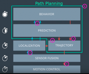
A path planner includes three main components: a vehicle predictor, a behavior planner, and a trajectory generator. Vehicle prediction involves estimating what other vehicles in the local environment might do next. Behavior planning decides what action to take next, given the goal and the estimates from the vehicle prediction step. Trajectory generation computes an actual path to follow based on the output from the behavior planning step.
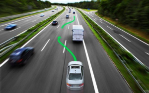
I created a vehicle path planner implementation which safely navigates a simulated vehicle around a virtual highway with other traffic. The vehicle attempts to keep as close to the speed limit as possible, while maintaining safe driving distances from other vehicles and the side of the road, and providing a comfortable riding environment for any passengers inside. This may involve switching lanes, passing vehicles, speeding up and slowing down.
Exploring my implementation
All of the code and resources used in this project are available in my Github repository. Enjoy!
Technologies Used
- C++
- uWebSockets
- Eigen
- Cubic Spline Interpolation
Path planning
Search and Cost Functions
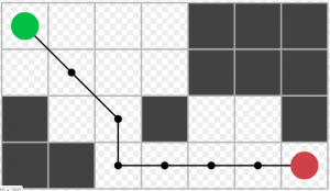
The fundamental problem in path planning is to find the optimal path from the start to the goal, given a map of the world, locations of all objects in the map, a starting location, a goal location, and a cost function. The “cost” in this case refers to the penalty involved in taking a particular path; for example, driving primarily on two lane 25 MPH roads to navigate between New York City and Los Angeles would have a high cost; most of the driving instead should occur on Interstate highways, which would have a much lower cost. Various actions that the vehicle can take incur different costs; left turns, right turns, driving forward, driving backward, stopping, and other actions will all incur costs, which may vary depending on the current speed or location of the vehicle.
Various algorithms exist for searching for a path; grid– and interval-based search algorithms (such as A*) are popular, and many other algorithms involving rewards or probabilistic sampling exist as well.
In reality, because the environment that an autonomous vehicle drives in is non-deterministic (other vehicles, road obstacles, and traffic markers may appear without warning), a path planner may choose to use a dynamic programming-based approach to plan for the optimal path to follow given multiple possible starting locations (called a policy).
Prediction
Prediction systems estimate what other vehicles will do in a given environment in the near future. For example, when a vehicle is detected by the perception systems, the prediction system would be able to answer “where will the vehicle to be in five seconds?” This happens by taking as input a map of the world and data from sensor fusion, and generating the future state of all other vehicles and moving objects in the local environment. Prediction systems generate multi-modal probability distributions, which means that the estimates they create may have multiple likely outcomes. Information about what vehicles generally do at certain locations in the world, coupled with the current and recent past behavior of a vehicle, inform the prediction to make certain outcomes more or less likely. For example, a car slowing down as it approaches a turn increases the likelihood of a turn.
Prediction algorithms can be model-based (where process models of vehicles are informed by actual observations) or data-driven (using, for example, a machine learning model to extract insight from raw sensor fusion data). Both algorithms have strengths: model-based approaches use constraints encoded in allowable traffic patterns and road conditions, while data-driven approaches may learn subtle nuances of behavior which may be difficult to model. Hybrid approaches, which use model- and data-based algorithms, are often the best to use. For example, the Gaussian Naive Bayes classifier is often used with appropriate features which are highly representative of specific trajectories to predict vehicle behavior.
Behavior Planning
Behavior planning answers the question of “what do to next” in an autonomous vehicle. Behavior planners use inputs from a map, route to destination, and localization and prediction information, and output a high-level driving instruction which is sent to the trajectory generator. Behavior planners do not execute as frequently as other autonomous vehicle systems (such as a sensor fusion system), partially because they require a large volume of input to generate a plan, but also because their output plans will not change as frequently as outputs from other systems. A behavior planner acts as a navigator, whose output might be “speed up”, or “get in the right lane”, including behaviors which are feasible, safe, legal, and efficient.
Behavior planners often use finite state machines, which encode a fixed set of possible states and allowable transitions between states. For example, when driving on a highway, the states might include “stay in lane”, “change to right lane”, or “get ready for left lane change”. Each state has a specific set of behaviors; for example, “stay in lane” requires staying in the center of the lane and matching speed with the vehicle ahead up to the speed limit. Selecting a new state from a given state requires a cost function, which allows for selecting the optimal state for driving to the goal. Cost functions often include as inputs current speed, target speed, current lane, target lane, and distance to goal, among others.
Trajectory generation
A trajectory generator creates a path that the vehicle should follow and the time sequence for following it, ensuring that the path is safe, collision-free, and comfortable for the vehicle and passengers. This happens by using the current vehicle state (location, speed, heading, etc), the destination vehicle state, and constraints on the trajectory (based on a map, physics, traffic, pedestrians, etc). Many methods exists for this: combinatorial, potential field, optimal control, sampling, etc. For example, Hybrid A* is a sampling method, which looks at free space around a vehicle to identify possible collisions, and is great for unstructured environments such as parking lots (without many constraints).
Polynomial trajectory generation works well for highways with more strict and predefined rules about how a vehicle can move on a road. A jerk (rate of change of acceleration) minimizing polynomial solver generates continuous, smooth trajectories that are comfortable for passengers. A jerk minimizing solver may take into account minimum and maximum velocities, minimum and maximum longitudinal (forward and backward) acceleration, maximum lateral (side-to-side) acceleration, and steering angle, among other inputs. Because the behavioral plan typically does not include an exact final state (speed, direction, location, etc), generating several similar concrete final states and computing jerk minimizing trajectories for all of them is typical. Then, the trajectory with the lowest cost which is drivable and does not collide with other objects or road boundaries is chosen. In this case, a cost function might include jerk, distance to other objects, distance to the center of a lane, time to the goal, or many other items.
Implementation
In this project, the goal is to safely navigate around a virtual highway with other traffic that is driving within 10 MPH of the 50 MPH speed limit and may change lanes (as other vehicles often do). The input provided is the vehicle’s localization and sensor fusion data, and there is also a sparse map list of waypoints around the highway. The vehicle should try to go as close as possible to the 50 MPH speed limit, which means passing slower traffic when possible. The vehicle must not collide with other vehicles, and must stay within lane lines unless going from one lane to another. Additionally, the vehicle should not experience total acceleration over 10 m/s^2 nor jerk that is greater than 10 m/s^3.
Vehicle prediction – Other vehicle tracking
The vehicle tracking section of code is responsible for using data from sensor fusion measurements to determine where other vehicles are relative to the controlled vehicle. This includes detecting vehicles directly to the left, ahead, and right and determining how much empty space exists between these vehicles. This information is used for the lane change decision making system.
Behavior planning – Lane change decision making
The lane change decision making system determines if the vehicle should attempt to change lanes if it is currently travellling at less than 90% of the maximum speed (50 MPH) and the vehicle is following less than 50 units behind the vehicle in front of it. Once that determination is made, the vehicle looks to both the left and right for an opening with no other vehicles. If both lanes are open, the lane with a vehicle farthest ahead is chosen for the lane switch.
Behavior planning – Speed control
The speed control system maximizes the speed in the current lane given traffic conditions. If no other vehicles are within 50 units ahead, the system accelerates slowly until almost 50 MPH is reached. Otherwise, the vehicle slows down to match the ahead vehicle’s speed, and maintains a distance from the ahead vehicle equal to the current velocity (a proportional following distance).
To achieve a constant following distance, a PID controller is used with proportional and differential controls turned on.
Trajectory generation
Once a target lane and velocity are computed, a trajectory is calculated several steps into the future. On a first trajectory generation run, the vehicle’s location and previous point using the vehicle’s yaw angle are computed; otherwise, the number of points remaining in the trajectory are obtained. Next, three points evenly spaced down the target lane are generated. These points are converted to x-y coordinates, and they are angle-corrected for the vehicle’s orientation in the environment. Spline interpolation is used for computing additional trajectory points, which when combined with any previous trajectory points from a previous iteration not traveled, to bring the total number of points up to 50. These points are then handed off to the simulator for the vehicle to follow.
Results
Using these components with input data from the simulator and existing map data, this path planner is able to drive the simulated vehicle safely and efficiently around the course, maximizing its speed while avoiding collisions. Simulation runs often approach hundreds of miles before any kind of collision is experienced, and multiple runs of the simulator show this very often due to unsafe and sudden behavior from other vehicles.
